5 Quantitative portfolio construction with ESG data and criteria

5.1 Simple portfolio choice solutions

ESG indicators are very well suited for portfolio integration and dozens, if not hundreds of articles have been written on this topic. We begin by mentioning a few papers that are very thoroughly written and provide the reader with a detailed account of the portfolio construction process. For instance, De and Clayman (2015) give a precise description of their methodology and report many results. They find that the best solution is to eliminate stocks from the lower tail of the ESG distribution. Oikonomou, Platanakis, and Sutcliffe (2018) test several quantitative methods (mean-variance, Black-Litterman, and robust estimation) and find that they work better than simple heuristic approaches (e.g., equally-weighted portfolios). Jondeau, Mojon, and Pereira da Silva (2021) argue that excluding a few heavy polluters is sufficient to drastically reduce the carbon footprint of benchmark portfolios. Alessandrini and Jondeau (2020) perform robustness checks across regions and sectors, but also compare best-in-class versus exclusion approaches. Lastly, Bruder et al. (2019) also look at the importance of regions and disentangle the three dimensions of ESG and their impact on returns and information ratios.

5.2 Improved mean-variance allocation

One common direction that is pursued by researchers is to integrate ESG scores directly in the utility function that the investor maximizes. This makes sense because, indeed, investors value sustainability and do obtain utility outside financial gains (see Bollen (2007), Riedl and Smeets (2017), Barber, Morse, and Yasuda (2021), Dyck et al. (2019), Hartzmark and Sussman (2019)). Thus, instead of maximizing expected returns for a given level of risk, agents may seek to maximize a combination between returns and weighted-average ESG scores. This simple idea is presented in Barracchini and Addessi (2012) and Gasser, Rammerstorfer, and Weinmayer (2017). Some variants of these methods are (in chronological order):

Table: Examples of ESG-driven portfolio optimization techniques

Reference	Contribution
Drut (2010)	proposes the maximization of a mean-variance utility, subject to a minimum level of aggregate ESG score.
Dorfleitner and Utz (2012)	introduce a utility function that is based on financial and sustainability returns of the portfolio.
Benedetti et al. (2021)	integrate views about carbon taxes within a Bayesian portfolio optimization problem.
M. Branch, Goldberg, and Hand (2019)	resort to optimized exclusion: they first shrink the investment set and then optimize on the remaining assets.
Fish, Kim, and Venkatraman (2019)	adjust returns with ESG metrics before they run optimizations (mean-variance and hierarchical risk parity).
Geczy, Guerard, and Samonov (2019)	implement the so-called APT Mean-Variance Tracking Error at Risk optimization.
Alessandrini and Jondeau (2020)	maximize the ESG rating of the portfolio under many constraints (related to benchmark tracking error, turnover, regional and industry exposition, etc.).
Bender et al. (2020)	add carbon constraints to their objective functions and show that it is possible to reduce the carbon emissions of portfolios without degrading the volatility of low-volatility portfolios.
M. Chen and Mussalli (2020)	propose to optimize the information ratio of a portfolio while integrating both alpha and ESG considerations.
Chan et al. (2020)	optimize a traditional quadratic utility function, but with constraints on factor exposures and with additional requirements on aggregate ESG and carbon scores.
Schmidt (2020)	minimizes the volatility minus the ESG score under a constraint of expected return.
Pedersen, Fitzgibbons, and Pomorski (2021)	the agent maximizes the Sharpe ratio of the portfolio for a given level of ESG score.
Geczy, Stambaugh, and Levin (2021) (originally written in the early 2000s)	focuses on allocations to mutual funds. The agent postulates a model for future returns and these models are subject to uncertainty, which is modelled in a Bayesian framework. The authors determine the financial cost of screening funds according to whether they are socially responsible or not. They provide some conditions under which this cost is high or low.
Coqueret et al. (2021)	propose to combine ESG attributes to other variables in the asset pricing literature (e.g., market capitalization or valuation ratios) to boost ESG-based optimization.
Alekseev et al. (2021)	hedge climate risk portfolios that mimic climate shocks. They test different definitions for these shocks and compare their mimicking portfolios to traditional sorts (narrative-based approach).
Fischer and Lundtofte (2021)	combine the DICE model (see Section 7.2) with Merton’s ICAPM to derive a four fund separation theorem.

A very favorable feature of most of these frameworks is that they often allow closed-form solutions that are easily implementable. Henceforth, we present the framework laid out in Pedersen, Fitzgibbons, and Pomorski (2021). For consistency purposes, we follow the notations of the model of Pastor, Stambaugh, and Taylor (2021b) (which is outlined below in Section 7.1.

The agent chooses an allocation \(w\) over \(N\) assets so that future wealth \(W_1=W_0(1+r_f+w'r)\), where \(r_f\) is the risk-free rate and \(r\) is the vector of returns of the risky assets. In addition to returns, assets are characterized by an observable ESG score g (which here has a vector form). The weighted average ESG score of the portfolio is thus \(\bar{g}=w'g/(w'1)\), where here \(1\) denotes a vector of \(N\) ones.³³ As is discussed in Section 3.1, the investor has preferences over both pecuniary and social performance, and seeks to solve the following program: \[\begin{equation} \underset{w}{\max} \left\{\underbrace{w'\mu - \frac{\gamma}{2}w'\Sigma w }_{\text{mean-variance}}+\underbrace{f\left(\frac{w'g}{w'1}\right)}_{\text{ESG tilt}}, \text{ subject to } w'1>0 \right\}, \tag{5.1} \end{equation}\] where \(\mu\) and \(\Sigma\) are the mean vector and covariance matrix of the returns \(r\), and \(f\) is the ESG preference function. As is customary, \(\gamma>0\) is the risk aversion parameter. The constraint \(w'1>0\) implies that the portfolio has a long-only bias, i.e., that long positions strictly outweigh short ones. Under additional factor assumptions, Varmaz, Fieberg, and Poddig (2022) show that it is possible to simplify this program to a plain quadratic optimization with linear constraints.

In traditional mean-variance analysis, the agent has the choice between fixing one level of average return and minimizing the volatility, or maximizing the average return of a given level of return dispersion. In the above formulation, there is one additional choice to make, and it relates to the average ESG score \(\bar{g}\). The efficient frontier is defined by maximizing the expected return under constraints \[\begin{equation} \max \left\{w'\mu, \ \text{subject to } \begin{array}{lll} w'1>0, & \text{leverage constraint}\\ \sqrt{w'\Sigma w} < \sigma_\text{target}, & \text{volatility constraint} \\ w'g > g_\text{target} & \text{ESG constraint} \end{array}\right\}, \tag{5.2} \end{equation}\] or minimizing volatility under constraints \[\begin{equation} \min \left\{ \sqrt{w'\Sigma w}, \ \text{subject to } \begin{array}{lll} w'1>0, & \text{leverage constraint}\\ w'\mu > \mu_\text{target}, & \text{return constraint} \\ w'g > g_\text{target} & \text{ESG constraint} \end{array}\right\}. \tag{5.3} \end{equation}\]

This implies that the frontier is a function of the target for the ESG score. This is shown in Figure , where we represent three different stylized frontiers. As the investor asks for a higher ESG score, the frontier shifts away from the unconstrained frontier and the investor must accept possibly lower returns and/or higher volatility.

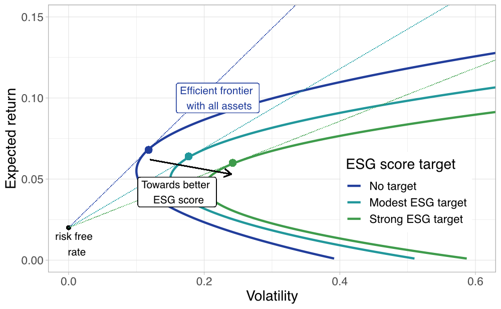
FIGURE 5.1: Stylized representation of ESG constrained frontiers. We present a diagram that depicts three efficient frontiers for various levels of targeted ESG score. The big dots at the intersection of lines and frontiers are the tangency portfolios

In a typical mean-variance optimization, the best portfolio is the one that maximizes the Sharpe ratio (tangency portfolio). It is thus useful to characterize the maximum Sharpe ratio that can be attained for a given level of aggregate ESG score: \[\text{SR}(\bar{g})= \underset{w}{\max} \left\{ \frac{w'\mu}{\sqrt{w'\Sigma w}}, \text{ subject to } \left[ \begin{array}{l} w'1>0 \\ w'g/(w'1)=\bar{g} \end{array} \right. \right\} .\]

In order to solve the original program defined in Equation (5.1), the agent must choose the following level of average ESG score: \[g^*=\underset{\bar{g}}{\max} \left\{\text{SR}(\bar{g})^2 +2\gamma f(\bar{g}) \right\}.\] The general solution to Equation (5.1) is a fund separation that reads:

\[\begin{equation} w^*=\gamma^{-1} \left( \underbrace{\Sigma^{-1}\mu}_{\text{TP}} + c_{\text{MV}} \underbrace{\Sigma^{-1} 1}_{\text{MV}} + c_{\text{ESG}} \underbrace{\Sigma^{-1}g}_{\text{ESG}}\right). \tag{5.4} \end{equation}\] The risky portion of the portfolio thus consists of three layers: the tangency portfolio (TP) which maximizes the Sharpe ratio, the minimum variance (MV) portfolio, and a so-called ESG tangency portfolio. The scaling constants \(c_{\text{MV}}\) and \(c_{\text{ESG}}\) can be found in the original paper.

5.3 Other quantitative techniques

Beyond simple extensions of mean-variance preferences, several papers have sought to resort to more complex optimization schemes and often solve them by means of fuzzy systems or genetic algorithms. We refer to the following list (chronologically sorted): Bilbao-Terol, Arenas-Parra, and Cañal-Fernández (2012a), Bilbao-Terol, Arenas-Parra, and Cañal-Fernández (2012b), Calvo, Ivorra, and Liern (2015), Bilbao-Terol et al. (2016) and Hilario-Caballero et al. (2020). In Li Chen et al. (2021), the authors resort to screening methods combined to ESG score and portfolio optimization. Likewise, Alessandrini and Jondeau (2021) propose a very exhaustive optimization scheme in which the ESG score is maximized, subject to a large palette of constraints: tracking error, turnover, regional and industry weights, factor exposure, and box constraints. The only drawback is the fundamentally black-box nature of the outcome.

Other contributions go even further and rely on systematic approaches, often linked to machine learning. For instance, Lanza, Bernardini, and Faiella (2020) compute brute force trees (test all combinations of ESG indicators) to derive the best possible portfolios. Likewise, Assael and Challet (2021) resort to boosted trees. In a similar fashion, Margot et al. (2021) derives an ad-hoc ML algorithm that tries to link ESG ratings to returns in a non-linear fashion. Goldberg and Mouti (2019) resort to supervised learning to predict maximum drawdown and find that ESG scores help improve the forecasting accuracy of the algorithms. Dash and Kajiji (2021) use ML to extract pervasive ESG factors and predict expected returns, which are then fed to a hierarchical multi-objective portfolio optimization model. Sokolov, Caverly, et al. (2021) mix natural language processing with Black-Litterman views to build ESG-tilted portfolios. J. Zhang and Chen (2021) combine screening, ML and portfolio optimization techniques to build efficient (green) equity portfolios in the Chinese stock market.

Lastly, though it does not refer to portfolio construction, but performance attribution, we mention the work of Bolliger and Cornilly (2021). The authors detail a methodology that aims to evaluate the carbon footprint of a portfolio. The authors contend that this can largely be driven by sectorial biases and that this dimension must be taken into account. Relatedly, Lo and Zhang (2021) outline a technique dedicated to evaluate the financial benefits (or harm) induced by sustainable investing. In their framework, the key quantity is the correlation between the impact factor (e.g., ESG score) of each stocks and their alpha (excess return in a factor model).

5.4 Miscellaneous tips, methods and other integration techniques

Statman and Glushkov (2016) find that the two main portfolio construction methods (ESG score screening and industry filtering) do not deliver the same results. They find value for the former but not for the latter. Mohanty, Mohanty, and Ivanof (2021) introduce ESG target. They construct overlays by over weighting stocks with higher ESG metrics until the portfolio improves its ESG score by 20% compared to a given benchmark. Gurvich and Creamer (2021) show that several carbon emission based sorts lead to various outcomes. Depending on whether portfolios are built on raw emissions (which introduces a size bias), emissions divided by market capitalization, or emissions divided by sales, the Sharpe ratios shift from good to outstanding.

B. Branch and Cai (2012) propose an original idea: build ESG portfolios that mimick the S&P 500. They show it is possible to deliver market performance with portfolios relying only on socially responsible stocks. Fan and Michalski (2020) improve momentum and quality factors with ESG screens and sorting procedures. Henriksson et al. (2019) introduce an original solution to overcome issues when firms do not have ESG ratings. They advocate the creation of an ESG factor (Good minus Bad) and the evaluation of each stock’s exposure to this factor. A loading significantly above zero should mean that the firm’s returns are positively driven by the ESG factor. At the aggregate level, the aim is to tilt portfolios toward good ESG proxies. Khan (2019) proposes a new methodology to construct robust governance and ESG scores that seem to do a good job at explaining returns. Palazzolo, Pomorski, and Zhao (2020) discuss the challenges in the crafting of carbon neutral portfolios.

In Widyawati (2020) (p. 633), the author makes the case that “there is little empirical knowledge about the most effective way to apply SRI as a quantitative financial model and how this application affects market equilibrium.” It seems more reasonable to conclude that there is a large body of empirical work, but the problem is that conclusions of some studies often contradict the findings of other analyses. There is no consensus on how precisely to efficiently integrate ESG ingredients in a portfolio strategy that performs well financially out-of-sample.³⁴ There is probably less uncertainty in the social good that comes from SRI, compared to its pecuniary benefits, although Cappucci (2018) warns against the perils of half measures that are only implemented for marketing purposes (see also Statman (2020) on this matter).

At an aggregate level, Harper (2020) provides some tips on how to integrate ESG criteria when searching and selecting an investment manager. Schoenmaker and Schramade (2019) draw the contours of an alternative investment paradigm for investors who seek long-term value creation. Cosemans, Hut, and Dijk (2021) specify a VAR model that includes temperature change as a predictor for (aggregate) equity returns. They estimate their model with a Bayesian method and subsequently maximize a constant relative risk aversion (CRRA) utility function based on these beliefs. Umar, Kenourgios, and Papathanasiou (2020) document that ESG indices are interconnected at the global level, thereby challenging the benefits of geographical diversification. Finally, Parker (2021) wraps the notion of impact investing in a goal-based allocation framework to help balance financial and sustainability targets.

One very interesting contribution is the work of Raynaud, Tankov, and Voisin (2020). The goal of the article is to articulate a methodology for portfolio managers who want to craft their allocation so as to participate to the global initiative toward the 2°C alignment (fixed by the 2015 Paris accord). The paper links climate metrics, macro-economics scenarios, and portfolio engineering in a non-technical and insightful fashion. For more details, the interested reader can have a peek at the alignment cookbook written by the authors. The assessment of the carbon footprint of portfolios, a material topic, is discussed in Erlandsson (2021).

Finally, the first issues of the Journal of Impact and ESG Investing are filled with various pieces of advice. For instance, Grim and Berkowitz (2020) provide general guidance when including ESG criteria in the investment process and mention a few use cases. Chan et al. (2020) show how to use intangible value and corporate culture proxies to improve the performance of more traditional factors (value and quality).