7 SRI in economic equilibria

Given its importance and relevance, SRI has recently seen a surge in theoretical contributions (though a few prescient researchers started working in this direction a few decades ago). We categorize the corresponding articles in two subgroups, though a few papers could belong to both categories. The first group (in Section 7.1 encompasses the papers that are more finance-driven and investigate the impact of ESG investing on asset prices. The second group (see Section 7.3 is more focused on economic policy and on the societal impact of SRI. The existing literature on the topic is extensive. The articles compiled in this chapter are a very incomplete snapshot of the research output on this domain.

Before we turn to the contributions, we propose a macro-view of the concepts of the field. First of all, humans enter the modelling process via four possible channels, which are depicted in Figure 7.1.

individuals, who either	inside firms, which	as part of government, which	inside lobbies,40 which
work for companies	require funding	is elected by individuals	may put pressure on firms
run companies	produce goods	regulates parts of the economy	can be funded by firms or by individuals
buy and consume products	may or may not pollute	collects taxes	may influence the government
pay taxes	may or may not seek high valuation (or, equivalently, seek to maximize profit)	may protect the environment
invest in firms	pay taxes

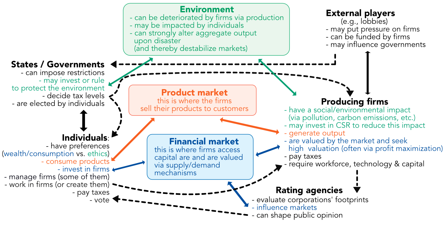
FIGURE 7.1: Theoretical framing. Diagram with the various forces at play in ESG investing

These four channels interact in (at least) three places. The first one is the product market, where firms sell goods that are bought by individuals. Firms may decide to shift product or policy to satisfy green-friendly buyers, though usually repercussing this choice in their prices. The second one is the financial market, where firms seek funding for their activities and where individuals and financial institutions allocate money in exchange of future payoff.

Finally, the last element, which is essential in ESG modelling, is the environment. It is given to humans; they exploit it, and by doing so, they alter it. But too much alteration may come with a cost: lower productivity (e.g., in agriculture), production shocks (linked to natural disasters), etc. Accordingly, taking care of it may be economically beneficial in the long run.

7.1 Asset pricing

We categorize models according to the number of agents in the economy.⁴¹ When only one agent takes part on the demand side, there are usually at least two firms, with differentiating postures with regard to ESG-related policy. And these postures affect their returns via some externality (e.g., climate change or tax shocks). When two or more agents participate, then their preferences toward sustainability are key: they usually have a choice between two (or more) profiles of firms and their demands for these firms’ shares will drive stock prices.

7.1.1 One agent

We begin a tour of models with only one agent below. The short summaries do not pretend to reflect the exhaustivity of authors’ contributions. Rather, we focus on some key points.

Albuquerque, Koskinen, and Zhang (2019) work with a representative agent who can invest in two types of firms (one standard and one producing CSR goods, thereby ensuring differentiation). One conclusion of the paper is that ESG-driven firms are expected to have a lower market beta (which is a proxy for risk), compared to traditional firms.

Karydas and Xepapadeas (2019) present an endowment economy with two jump-diffusion Lucas trees (general versus brown, the latter being carbon intensive). Two sources of shocks are present in the economy that drive asset returns: environmental and macro-economic. The representative agent has Epstein-Zin preferences. The authors derive the values of the risk-free rate and an expression for the equity premium.

Bansal, Kiku, and Ochoa (2019) find that aggregate consumption growth is impacted by climate change damages. In their economy, the representative agent has Epstein Zin preferences. There exists a feedback loop: economic growth, via industrial emissions, increases global temperatures, which, in turn, may shock the growth. Temperature evolution has two random components, one that is exogenous and one that stems from economic activity. One key result is that these two components naturally drive the log of average returns of all assets.

Colonnello, Curatola, and Gioffré (2019) introduce an economy with two firms (one responsible, and another one: the sin company). The representative agent derives utility from dividends and from the ethicality of the firm they receive these dividends from. As long as ethicality is positively perceived, the ethical firm has a higher price, compared to the sin firm.

P.-H. Hsu, Li, and Tsou (2021) propose a general equilibrium model in which governments decide at some point in time to implement a policy change which is environmentally friendly. Agents are represented by a continuum of identical households. One asset pricing implication of the model is: “agents demand a positive compensation for their exposures to such a regime change shock.”

The model of Campbell and Martin (2021) focuses on a representative agent who has to allocate her wealth between two assets: one risky, one riskless. In this paper, sustainability is defined in a different fashion, compared to other articles. The authors view sustainability as the opportunity to sustain expected utility, so that the agent makes choices that would ensure that her descendants experience a utility that is not lower than hers. Under independent and stationary returns, the authors show that the sustainable social rate of time preference and the consumption-wealth ratio are equal and lie between the risk-free rate and the risky return.

7.1.2 Two or three agents (or agent types)

We then proceed to models with two agents. In Heinkel, Kraus, and Zechner (2001), the framework relies on an economy with 3 types of firms (acceptable (ESG friendly), unacceptable (polluting) and “reformed” (i.e., operating an ESG shift)), as well as on two types of agents, one of which refuses to hold assets of unacceptable firms - by operating a green screening before investing. All agents have preferences defined by constant absolute risk aversion (CARA) utility functions. The authors derive the equilibrium prices of the three firms and show that the price of acceptable firms does not depend on the proportion of green investors.

H. L. Friedman and Heinle (2016) lay out a two-period economy in which two types of investors allocate between one risk-free asset and one producing firm (which yields two outputs: one cash-flow and one CSR externality). One investor type is only sensitive to cash flows, while the other cares about both corporate outputs. The authors derive a simple form for the equilibrium price with two terms, one being the theoretical price in the absence of CSR-driven investors.

In H. A. Luo and Balvers (2017), normal investors are opposed to boycotting investors. It is shown that the average excess return has two components: one related to the market factor, the other to the boycott factor. Zerbib (2020) works with a single period, and three investor types (one regular mean-variance optimizer and two that are ESG-driven who exclude some assets). The author derives a formula for average returns. Rosenlund Soysal and Lessmann (2020) studies buyback mechanisms for firms in a model in which two investors disagree about market expectations. The authors compare this disagreement with nuances in operators that price climate risk for fossil fuel companies, in which buybacks are common practice.

In Goldstein et al. (2021), there are two agent types (traditional versus green) and two assets: a risk-free bond with fixed certain payoff and risky stock which yields two outputs: a monetary component (akin to a cash-flow) and a social or environmental component (e.g., pollution). Both agent types have CARA preferences over a weighted sum of both components. Via a simple market clearing assumption, the authors prove that multiple equilibria may arise, and the paper describes the properties of these equilibria.

7.1.3 Many agents

To conclude this section, there are also some contributions with many heterogeneous agents. In Pastor, Stambaugh, and Taylor (2021b), there is a continuum of agents who differ in their inclination towards sustainability. This model is simple and provides intuitive results, thus we detail it in more depth. \(N\) firms, henceforth indexed by \(n\), yield both excess returns \(r_n\) and societal impacts (\(g_n\), measured by some binary (green versus brown) observable ESG proxy). Agents obtain utility both from these returns and from non-pecuniary benefits stemming from the positive impacts of the firms they invest in. More precisely, their portfolio composition is a \(N\times 1\) vector \(X_i\), so that their wealth at time \(1\) satisfies \(W_{1,i}=(1+r_f+X_i'r)\), where \(w_{0,i}\) is the wealth at time \(0\). The utility (value) function for each agent reads: \(V(W_{1,i},X_i)=-e^{-A_iW_{1,i}-d_ig'X_i}\), where \(A_i\) is the risk aversion coefficient of agent \(i\) and \(d_i\) proxies his taste for ESG. The vector column \(g\) stack all \(g_n\) scores. In addition, the vector of all returns satisfies \(r=\mu + \epsilon\), where \(\mu\) contains the mean excess returns and \(\epsilon\) is a noise term that follows a Gaussian law with covariance matrix \(\Sigma\). The first important result is that the optimal allocation for agents is given by \[X_i = \frac{1}{A_iW_{0,i}}\Sigma^{-1}\left(\mu + \frac{1}{a_iW_{0,i}}b_i \right),\] and for analytical tractability, the authors assume that \(A_iW_{0,i}=a\), so that all relative risk aversions are equal. Relative wealths are given by \(\omega_i=W_{0,i}/W_0\), where \(W_0\) is the aggregate wealth at time 0. Notably, the market clearing condition imposes that the market portfolio, written \(w_m\), satisfies \[\mu = a \Sigma w_m-\frac{\bar{d}}{a}g,\] where \(\bar{d}=\int_i \omega_id_idi\) is the wealth-weighted average of ESG tastes (across agents). The market equity premium is then \(\mu_m=w_m'\mu\). One major result of the paper is that the equilibrium value of excess return is \[\mu= \frac{ \mu_m }{w_m'\Sigma w_m} \times \Sigma w_m - \frac{\bar{d}}{a}g,\] where the second term highlights the departure from the CAPM that comes from the ESG-driven preferences. Importantly, if the aggregate preference \(\bar{d}\) is strictly positive, then the expected return of stock \(n\) decreases with its ESG score \(g_n\) and its CAPM alpha is \(- \bar{d}g_n/a\). In Berg, Kölbel, and Rigobon (2022), the expected return is also negatively and linearly link to the ESG score or signal.

In Pedersen, Fitzgibbons, and Pomorski (2021), similar derivations are found. The framework is different, as ESG scores reveal information on dividend flows. In addition, there are three types of investors: those who ignore ESG data, those who exploit ESG scores but do not care about sustainability, and those who value sustainability and prefer high ESG firms. The expected return of stock \(n\) (given \(g\)) is \(\mu_n=\beta_n\mu_m-c(g_n-g_m)\), where \(\beta_n\) is the beta of asset \(n\) with respect to the market (which has expected return \(\mu_n\)). \(g_n\) and \(g_m\) are the ESG scores of asset \(n\) and the market, respectively. The constant \(c\) relates to \(c_{\text{MV}}\) and \(c_{\text{ESG}}\) in Equation (5.4) from Chapter 5. The paper by Pastor, Stambaugh, and Taylor (2021b) contains many other theoretical predictions. Among those, the authors postulate that if ESG concerns increase unexpectedly, green assets can outperform.

This latter claim is empirically tested in Ardia et al. (2020) (with positive results). Finally, Avramov, Cheng, et al. (2021) generalize the previous approach by incorporating volatility in ESG metrics (see also Berg, Kölbel, and Rigobon (2022)). Indeed, one key ingredient is the ESG score that is used by investors to allocate their wealth. In Pastor, Stambaugh, and Taylor (2021b), it is directly observable, without ambiguity, whereas in practice, several rating agencies may disagree on the matter (see Section 2.2). Thus, one important quantity is the volatility of this score, which serves as proxy of disagreement on the ESG virtue of a given firm. In Avramov, Cheng, et al. (2021), the authors derive optimal strategies and equilibrium expected returns under general forms of cross-asset disagreement. They show that volatility in ESG scores can alter the vector of expected returns \(\mu\) and that in some particular cases, green firms can have alphas that are larger than those of brown firms. Empirically, Christensen, Serafeim, and Sikochi (2021) find that higher disagreement increases stock return volatility.

7.2 The DICE models

Classical references for the economic effect of global warming are the books by the 2018 Nobel Prize recipient, William Nordhaus: W. D. Nordhaus (1994), W. D. Nordhaus and Boyer (2000), W. D. Nordhaus (2014); see also the recent overview of W. Nordhaus (2019). Recent contributions and research directions are surveyed in Farmer et al. (2015). One of the central models of Nordhaus, the DICE (Dynamic Integrated Climate-Economy) model, has been extended (e.g., with Epstein-Zin preferences in Ackerman, Stanton, and Bueno (2013) or with stochastic productivity in Yongyang Cai and Lontzek (2019)). Robust simulations of DICE models are outlined in Hu, Cao, and Hong (2012) for the purpose of evaluating global warming policies. Two important references are the book by Stern and Stern (2007) (see Stern (2008) for a short version) and the survey by Pindyck (2013). DICE models belong to the larger class of Integrated Assessment Models (IAMs). The article by D. Diaz and Moore (2017) provides a short and accessible overview of some of these models.

Because of its importance, we briefly summarize the DICE model below. There have been many versions thereof, and the one we present stems from W. D. Nordhaus (2017). The focal quantity in the model is the total welfare, computed over a finite time horizon:

\[\begin{equation} W=\sum_{t=1}^T U(c_t)L_tR_t, \tag{7.1} \end{equation}\] where \(U\) is a utility function (taken to be of CRRA type: \(U(c)=u^{1-\alpha}/(1-\alpha)\)), \(c_t\) is per-capita consumption, \(L_t\) is population (labor). Total consumption is \(C_t=c_tL_t\). \(R_t=(1+\rho)^{-t}\) is the discount factor on welfare (\(\rho\) being the pure rate of social time preference). In all studies, \(\rho\) is taken to be between 0 and 3% (see Adler et al. (2017)). Total consumption is linked to net output \(Q_t\) and investment \(I_t\) by \(Q_t=C_t+I_t\) and \[\begin{equation} Q_t=\Omega_t(1-\Lambda_t)Y_t, \tag{7.2} \end{equation}\] where \(Y_t\) is gross output and \(\Omega_t\) and \(\Lambda_t\) are the damage and abatement-cost functions, respectively. The former is further decomposed into \(\Omega_t=D_t(1+D_t)^{-1},\) with \[\begin{equation} D_t=\psi_1 TAT_t+\psi_2TAT_t^2, \tag{7.3} \end{equation}\] where \(TAT_t\) is the total average temperature change. This implies that economic damage is proxied by a quadratic function of temperature change.

One important driver of global warming is the emission of carbon gases. In the model, total CO\(_2\) emissions are written as \(E_t\) and they are an affine function of gross output \(Y_t\): \[\begin{equation} E_t=\sigma_t(1-\mu_t)Y_t+E_t^{\text{exo}}, \tag{7.4} \end{equation}\] where \(\sigma_t\) is carbon intensity, \(\mu_t\) is the emissions-reduction rate, and \(E_t^{\text{exo}}\) stands for exogenous land emissions. The DICE model then has a climate component that maps the carbon emissions \(E_t\) into global temperature changes: \[\begin{equation} TAT_t=f(E_t, TAT_{t-1}, Z), \tag{7.5} \end{equation}\] where \(Z\) are other variables, including greenhouse gas emissions, radiative forcings, and ocean temperatures. A macro-view of the model is presented in Figure 7.2.

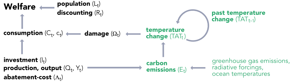
FIGURE 7.2: DICE model: simplified representation. Diagram summazing the DICE model. Grey components stand for the climate parts/variables of the model

The social cost of carbon (SCC) is formally defined as:

\[\begin{equation} SCC = \frac{\frac{\partial W}{\partial E_t}}{\frac{\partial W}{\partial C_t}}=\frac{\partial C_t}{\partial E_t}, \label{eq:scc} \end{equation}\] which equals the ratio of the marginal welfare impact of time-\(t\) emissions to the marginal welfare impact of a unit of time-\(t\) aggregate consumption.⁴² The second equality simplifies this to the economic impact of a unit of emissions in terms of consumption. The SCC can typically be expressed in dollars (numerator) per metric tons of CO\(_2\) (denominator). Given the large number of variables entering the model, differences in estimates yield various outcomes, and SCCs are documented to vary across time (moments when calibrations are performed) and models (see, e.g., W. D. Nordhaus (2017)). Some researchers even propose alternative definitions, e.g., that are corrected for some risks (Bremer and Ploeg (2021)).

The SCC can of course be estimated for different geographical zones. The European Union and the US often have similar costs, with China often ranking first. Rather surprisingly, the estimates of the cost of carbon are stable over different periods (Tol (2021a)). We refer to Auffhammer (2018) for a survey on the economic costs of global warming.

Countries are not equally armed to cope with the consequences of climate change (see, e.g., Semieniuk and Yakovenko (2020)} for a discussion on disparities in emissions across countries). Mealy and Teytelboym (2020) develop a model that quantifies the ability of economies to adapt their production capabilities to match new demands and increase green exportations. Germany, in particular, seems well equipped.

Finally, there have been recently researchers that have argued that cost and damage estimates from the economic literature are vastly underestimated. Steve Keen (2020) and Stephen Keen et al. (2021) belong to this category.

7.3 Other models for social impact

7.3.1 One agent

In line with Section 7.1, we organize a review of other contributions according to the number of agents in the models. We start with single agent theories. In Daniel, Litterman, and Wagner (2018), the authors apply ideas from asset pricing to a climate change problem. The representative agent optimizes the trade-off between the known cost of mitigating the risks of global warming and the unknown benefits that will result from this mitigation. Dam and Heijdra (2011) resort to a continuum of households, but they are identical. The authors study the impact of abatement policies and socially responsible investing on the environment.

Barro (2015) quantifies the impact of rare disasters on GDP output. The model incorporates a representative household (with Epstein-Zin preferences over consumption, which is a portion of GDP), a benevolent government. This government invests to reduce the odds of an environmental catastrophe. After calibration, the author concludes that the optimal level of investment in the environment (by the government) can be a sizable proportion of the GDP.

In the model of Kaul and Luo (2018), a for-profit firm competes with a non-profit organization (NPO). Both provide a social good, but only the former produces (and sells) a consumer good (which is bundled with the social good). A representative consumer may give money to the NPO, or buy a product from the firm, but derives utility from social contributions only. The authors different configurations of their model (i.e., alternative parametrizations), which notably relate to corporate philanthropy, greenwashing and shareholder activism.

The article by Yongyang Cai and Lontzek (2019) evaluates the impact of climate risk on the economy. The climate side is modelled by three components: carbon emissions, temperature growth and a third factor, which is a tipping element and models irreversible changes. The economic side is an adaptation of the DICE model developed by Nordhaus (see, e.g., W. D. Nordhaus (2014)). Two novel features are the introduction of Epstein-Zin preferences and the randomness of the productivity process. The main contribution is to link the so-called social cost of carbon to economic risks and climate risks.

Hambel, Kraft, and Ploeg (2021) model a production economy with two industries (one green (carbon-free) and one polluting). The representative agent allocates wealth between these two industries. The production output is impacted by rising temperatures. Global warming also penalizes the growth rate of capital and may lead to macro-economic disasters. The paper derives several theoretical results and gives the dynamic of the stochastic discount factor as well as the value of the risk-free rate.

In H. G. Hong, Wang, and Yang (2021), a representative agent (which represents both public and private investors) can invest in three types of assets: green stocks, brown stocks and a riskless bond. In addition, the agent may invest in insurance claims for disasters. This agent, because it cares about the future, is bound to spend a given proportion \(\alpha\) of total wealth in green stocks. Firms qualify as sustainable only if they spend a minimum amount on disaster risk mitigation (e.g., on decarbonization technologies). In equilibrium, the agent does not hold any positions in bonds. In addition, after a calibration of their model, the authors discuss realistic values for \(\alpha\). The levels they discuss are quite high, ranging between 36% and 78%. This can be interpreted as a strong call for SRI.

7.3.2 Two agents

We then summarize a few articles that involve two agents. In Baron (2009), a continuum of citizens invest in two firms, one of which is morally motivated, while the other is not. The citizens also buy the products of these companies. Firms may face social pressure from an external activist who attacks reputation. The main result of the paper is that the moral firm sells its products at a premium and targets a clientele who values CSP. Under some technical assumption, this firm may be more profitable than the self-interested firm. Oehmke and Opp (2020) devise a production economy financed by two types of investors (normal versus ESG driven). In the paper, firms resort to two possible technologies (one clean, one polluting). We quote one of their conclusions:“if the entrepreneur and socially responsible investors jointly internalize all externalities, production will always be clean.”

In De Angelis, Tankov, and Zerbib (2022), the market comprises many companies, and there are two investor types (regular and green). The latter takes into account environmental externalities in their forecasts of dividends (future cash flows). Companies choose their carbon emissions so as to maximize their market value, but reducing emissions is costly. Two simple conclusions are: (i) prices depend heavily on (the sign of) externalities and (ii) emission reduction depends on a trade-off because of externalities and is also impacted by the proportion of green investors.

The model of Landier and Lovo (2020) presents two types of agents (capitalists and entrepreneurs) who consume two types of goods, the production of which generates pollution. Agents benefit from consumption, but suffer from production. Capitalists can invest in three funds: one related to the two industries (stemming from the two products) and one that is ESG driven. Upon equilibrium in the model, one surprising finding is that all funds have the same return. Another interesting finding is that in order to be impactful, the ESG fund must invest a minimal amount of money in a given industry.

The article of Mackey, Mackey, and Barney (2007) introduces an economy in which \(N\) firms sell the same product and generate the same earning. Their goal is to maximize their value. The only differentiating element is the amount they are willing to invest in socially responsible activities which do not generate revenue. On the other side of the market are two types of investors, namely those who are pure profit maximizers and those who only invest in SR firms. The core equilibrium property of the paper is that the proportion of green investors is equal to the proportion of green firms.

Gupta, Kopytov, and Starmans (2021) propose a theoretical model to assess the speed with which investors are likely to influence a firm’s negative externalities. A firm owner faces two investor types (traditional versus sustainable). Counter-intuitively, the model predicts that the presence of green investors may delay the reduction of the social cost of production.

Finally, in D. Green and Roth (2020), there are three types of agents: commercial, values-aligned social, and sophisticated social. Commercial investors care only about return on capital. Values-aligned social investors care about capital returns as well as the social welfare stemming from their own investments. Sophisticated social agents derive utility from capital gains and from the aggregate social welfare (created by all entrepreneurs who receive funding from all agents). The authors derive theoretical properties of equilibria in their model. In particular, they pinpoint the flaws in values-aligned investors. Typically, the decisions of the latter can always be altered to improve total welfare. In addition, in welfare-optimal equilibrium, some values-aligned investors could be switched into sophisticated investors and receive higher returns, while at the same time increasing total welfare.

An interesting question is raised in Hakenes and Schliephake (2021): is it more important or efficient to invest sustainably, or to consume responsibly? The authors show that, in fact, both have similar effects and that what matters most is the targeted impact of households, i.e., the intensity with which they wish to attain sustainable goals.

7.3.3 Further contributions

The final part of the survey is dedicated to original contributions which are not best categorized according to the number of agents they consider. The technical article of Baron (2008) shows how individuals can drive CSR. They are viewed as customers, investors and possible firm managers, and these three channels can impact firm value and social output. In a similar vein, Baron (2007) considers agents who create or invest in two types of firms: classical profit maximizers versus CSR driven. Their preferences encompass both consumption and social dimensions. Citizens derive social satisfaction from two channels: via the shares they own from CSR firms, or from direct personal giving to social causes (this is inspired from Zivin and Small (2005)). Among many theoretical insights, the author shows that creating CSR firms increases social giving and that tax benefits may favor CSR firms to the point that their values surpass those of their non-CSR competitors.

In Nutz and Stebegg (2021), game theory is used to elaborate an equilibrium among firms that decide production levels and technology types subject to uncertainty on the transient climate response (TCRE) which links temperature changes and carbon emissions.

The article by Moisson (2020) has many theoretical implications. The model assumes two production technologies (green and brown) compete for capital. The latter generates negative externalities. A continuum of investors have three drivers: motivation for the common good, image concerns, and pecuniary incentive (because green portfolios may shrink consumption levels). The author derives conditions for the positivity of the green premium and analyzes the impact of taxes that would penalize brown savings. Among other topics, the author discusses the dichotomy between best-in class versus exclusion strategies and the efficacy of shareholder activism. Monetary and policy issues are theoretically tackled in Böser and Colesanti Senni (2020): the authors show that a transition to a low-carbon economy is possible by incentivizing banks via emission-based interest rates.

In a different spirit, the study of Chowdhry, Davies, and Waters (2019) is project-driven. The project requires financial and labour supply and generates monetary and social payoffs. The authors discuss the impact of the agents’ preferences. One optimal combination is when the manager (who supplies the workforce) is agnostic about social goals, but is also funded by a socially concerned investor.

Edenhofer, Lessmann, and Tahri (2021) model the economy and the decision processes between a government, a representative household and a long term investment fund. They resort to game theory and propose a game between the regulator and the household. The former sets a carbon budget but may change its mind subsequently (because of a commitment problem), while the latter must invest by guessing the final (ultimate emission budget). The authors show that there are two Nash equilibria in this game; one is ambitious in terms of emission abatement, and the other is not.

Finally, we mention the work of Alvarez and Rossi-Hansberg (2021). The authors build a huge theoretical representation of the world, involving topics like technology, trade balance, carbon cycles, temperatures and natality rates. Given a calibration of their model and specific scenarios, they evaluate the local impact of climate change for every region of the world, at a very granular level. They conclude that while most of the world (especially Africa and South America) will suffer from global warming, some (currently cold) regions, like Siberia, Canada, and Alaska, may benefit from it.

7.4 Uncertainty

We end our summary with a very thoughtful contribution. M. Barnett, Brock, and Hansen (2020) take a step back and reflect on modelling issues that researchers face when crafting theories on climate change and its impacts. The key notion is uncertainty, because the randomness of the physical phenomena at play, and the errors researchers make when modelling them, can often be overlooked, or underestimated. The authors show that uncertainty is a major risk which can bear profound social costs. They list three levels of uncertainty:

• Risk. Any given model incorporates randomness because predictions are always false. Errors and/or innovations are always characterized by some statistical distribution. Most of the time, these distributions are only known after a model has been estimated.
• Ambiguity. Policymakers and investors can decide to consider several models. Some models may be more or less optimistic or conservative, and thus be associated to more or less favorable scenarios. However, it is impossible to know which ones are more likely, and agents must weight these models in order to make a final decision. Ambiguity pertains to the uncertainty across these models.
• Misspecification. Models are simplified and imperfect representations of the real world. The errors that they make are only known via past data. How models behave in the future (their generalization ability) is also subject to uncertainty. This can be defined as misspecification risk.

In a follow-up paper, L. P. Hansen (2021) adresses the implications of climate change for central banks’ policies. Some of these concepts are also studied in Yongyang Cai (2020) and Manski, Sanstad, and DeCanio (2021).