4 ESG investing and financial performance
One of the central questions in ESG investing pertains to its opportunity cost: is sustainable investing penalizing from a pure pecuniary standpoint? This chapter addresses this complex and highly debated question. We start by a simple model that illustrates some typical mechanisms that can enlighten the situations when green firms can outperform brown ones. Then, we split the contributions of the impact of ethical screens on financial performance into four categories: the ones that document a positive relationship, the ones that find a negative relationship, the ones that report no particular relationship, and finally the ones that conclude that the relationship is contingent on some external factors. We mostly refer to financial performance in the sense of returns, though sometimes it means valuation. Nevertheless, SRI impacts other aspects of corporations’ finances, with risk being a major concern. We list some of these facets in the last two subsections below.
While the purpose of this chapter is to study the link between sustainability choices and financial performance, we do it in one direction (from ESG to finance). DasGupta (2021) has shown that mediocre financial performance can be an incentive for firms to improve their ESG practices.
4.1 Toy model
The mathematics-averse reader is advised to skip this subsection.
4.1.1 Theory: assets, agents, equilibrium
A full section of the survey is dedicated to theoretical models (Chapter 7), so the framework we present here is very stylized.24 We consider two agents and two risky assets (for simplicity). The two assets are indexed by \(g\) for green and \(b\) for brown, while the two agents are indexed with uppercase letters \(G\) (sustainability sensitive agent) and \(B\) (less ESG-driven, or even ESG insensitive agent). We will often use \(X\) to denote one of the agents (\(G\) or \(B\)) and \(y\) one of the assets (\(g\) or \(b\)).
Assets. Prices are denoted with \(p_g\) and \(p_b\). Both assets are expected to yield a cash-flow (or payoff): \(z_g\) and \(z_b\), respectively, and we assume that they have a correlation equal to \(\rho\). Agents agree on the variances of these payoffs, \(\sigma_g^2\) and \(\sigma_b^2\). However, they are allowed to disagree on their means: agent \(G\) estimates they are \(m_{Gg}\) and \(m_{Gb}\) while agent B believes they are \(m_{Bg}\) and \(m_{Bb}\). The assets are also characterized by a non-random (observable25) ESG score: \(e_g\) and \(e_b\), such that, naturally, \(e_g>e_b\). Both assets have fixed supplies \(s_g\) and \(s_b\), which are supplied by so-called noise traders who trade for reasons other than payoffs. One risk-free asset is also available in unlimited supply, with unit price and certain payoff equal to \(r>0\).
Agents. Agents have initial wealth \(W_G\) and \(W_B\), for the Green (sustainability-driven) and Brown agent, respectively. Each agent \(X\in \{G,B \}\) buys a quantity \(q_{Xy}\) of shares of asset \(y\in \{g,b \}\). The terminal wealth of agents satisfies \[W_X^*=\underbrace{r(W_X-q_{Xg}p_g-q_{Xb}p_b)}_{\text{payoff from riskless asset}}+\underbrace{q_{Xg}z_g+q_{Xb}z_b}_{\text{payoff from risky assets}}, \quad X\in \{G,B \} .\] We re-write this expression in the form of the gross return: \[\frac{W_X^*}{W_X}=r(1-w_{Xg}p_g-w_{Xb}p_b)+w_{Xg}z_g+w_{Xb}z_b, \quad X\in \{G,B \} ,\] where \(w_{Xy}=q_{Xy}/W_X\) is the number of shares of agent \(X\) in asset \(y\), divided by the total initial wealth of the agent.26 Also, the ESG score of agent \(X\)’s holdings is evaluated as \[E_X=w_{Xg}e_g+w_{Xb}e_b.\] The agents have a quadratic utility on gross return on wealth, plus an ESG component: \[U_X=\mathbb{E}\left[\frac{W_X^*}{W_X}\right]-\frac{\gamma}{2}\mathbb{V}\left[\frac{W_X^*}{W_X}\right]+\delta_X E_X,\] where \(\delta_G>\delta_B\) means that agent \(G\) cares more about ESG score than agent \(B\). The risk aversion coefficient \(\gamma>0\) is common to both agents. If we use bold vector notations for prices \(\textbf{p}=[p_g \ p_b]\) and relative portfolio holdings \(\textbf{w}_X=[q_{Xg} \ q_{Xb}]\), then the utility function reads \[U_X=r-r\textbf{w}_X'\textbf{p} +\textbf{w}_X'\textbf{m}_X-\frac{\gamma}{2}\textbf{w}_X'\boldsymbol{\Sigma}\textbf{w}_X+\delta_X\textbf{w}_X'\textbf{e},\] where \(\textbf{m}_X=[m_{Xg} \ m_{Xb}]'\), \(\textbf{e}=[e_g \ e_b]'\) and \(\boldsymbol{\Sigma}=\begin{bmatrix} \sigma_g^2 & \rho \sigma_g\sigma_b \\ \rho \sigma_g\sigma_b & \sigma_b^2 \end{bmatrix}.\) The first-order condition (the gradient of \(U_X\) must be equal to zero) implies \[-r \textbf{p}+ \textbf{m}_X-\gamma \boldsymbol{\Sigma} \textbf{w}_X+ \delta_X \textbf{e}= \textbf{0},\] so that agents’ relative demands satisfy \[\begin{equation} \textbf{w}_X=\gamma^{-1}\boldsymbol{\Sigma}^{-1}(\textbf{m}_X+\delta_X\textbf{e}-r\textbf{p}) . \tag{4.1} \end{equation}\] As \(\delta_X\) increases in magnitude, the agent will progressively grant more importance to the ESG score \(\textbf{e}\) than to the expected payoff \(\textbf{m}_X\). Also, all other things equal, the magnitude of demand decreases with risk aversion and payoff volatility. Note that the demand can very well be negative. Also, if the correlation between payoffs (\(\rho\)) is zero, the expression simplifies to \[\begin{equation} \hspace{18mm}w_{Xy}=\frac{m_{Xy}+\delta_Xe_y-rp_y}{\gamma \sigma_y^2}, \quad X\in\{G,B\}, \quad y \in\{g,b \}. \tag{4.2} \end{equation}\] There are three parts in the above formula. The first can be interpreted as the agent-specific attractiveness of the asset \(m_{Xy}+\delta_Xe_y\), which has two components: payoff and sustainability. The second is the negative impact of the price (demand decreases with price). The third (denominator) is risk. The assumption that \(\rho=0\) is quite strong, as it implies that both assets are priced independently.
Equilibrium. The price-weighted demands must satisfy the market clearing condition (demand equals supply). The aggregate demand for one asset \(y\) is simply \((q_{Gy}+q_{By})p_y\), i.e., the price times the total holdings (in shares). In our simple setting, we assume a vector \(\textbf{s}=[s_g \ s_b]'\) of supply for assets, thus \[\begin{equation} \underbrace{\text{diag}(W_G\textbf{w}_{G} +W_B \textbf{w}_{B})\textbf{p}}_{\text{total demand for asset }}=\textbf{s}, \tag{4.3} \end{equation}\] where diag\((\textbf{v})\) takes a vector \(\textbf{v}\) as argument and yields a diagonal matrix with \(\textbf{v}\) as diagonal values. The above equation highlights the importance of each agent’s relative weight on the market, which is given by the ratio of their wealth to total wealth \(W=W_G+W_B\). To further ease the analysis, we posit that the correlation between payoffs is zero. Consequently, plugging the demands in Equation (4.2), the equation for asset \(y\) translates to \[-\overbrace{[r\left(W_G+W_B\right)]}^{\text{riskless alternative}}p_y^2 +\overbrace{ \left[W_G(m_{Gy}+\delta_Ge_y)+W_B(m_{By}+\delta_Be_y)\right]}^{A_y=\text{total weighted attractiveness}}p_y-\overbrace{\gamma \sigma_y^2s_y}^{\text{risk/supply}}=0,\] where we have singled out the total attractiveness of the asset, which we write \(A_y\). The equation is quadratic in the price \(p_y\) because of the way the \(w_Y\) are defined. In many papers, the market clearing Equation (4.3) leads to linear forms. Under the parametric condition \[\begin{equation} (\textbf{C}) \hspace{6mm} A_y^2-4\gamma \sigma_y^2s_yrW\ge0, \label{eq:assumpA} \end{equation}\] the positive price of asset \(y\) is \[\begin{equation} p_y = \frac{\sqrt{A_y^2-4\gamma \sigma_y^2s_yrW}+A_y}{2rW}. \tag{4.4} \end{equation}\] Intuitively, the price of an asset is increasing in attractiveness, and decreasing with risk and supply.
4.1.2 Numerical example
Now, let us test some parametric configurations of the model so as to reveal several key theoretical predictions. We make the following simplifications:
- We normalize wealths. \(W_B=1\), so that the Brown investor is the benchmark. We can take several values for \(W_G\). For \(W_G=0.5\), the Green investor represents one third of the market and for \(W_G=2\), two-thirds of the market.
- For ease of interpretation, we fix the ESG scores to \(e_g=1\) (green) and \(e_b=0\) (brown). Also, for both assets, \(\sigma_y=0.2\) (\(\sigma_y^2=0.04\)) and \(s_y=1\) (unit supply).
- The taste for sustainability of the Green investor is set to \(\delta_G=0.15\). On the other hand, the Brown investor does not care about ESG and \(\delta_B=0\).
- Finally, we assume that \(r=0.02\). \(r\) has two important effects on prices. First, it plays a scaling role in condition (\(\textbf{C}\)): large values of \(r\) may lead to a violation of the condition. Second, it normalizes price values in Equation , so that, at a first-order approximation, prices are inversely proportional to \(r\).
We consider two alternative versions of agent beliefs:
- Extreme polarization. The Green investor is purely driven by ESG concerns and is agnostic with respect to returns, so that \(\textbf{m}_G=\textbf{0}\). The Brown investor, in contrast, and as is commonly accepted (see Bolton and Kacperczyk (2021), Bolton and Kacperczyk (2020)), expects incremental returns for the brown asset (akin to a carbon premium). We model that by assuming that \(\textbf{m}_B\) is negatively linked to \(\textbf{e}\): \(m_{Bg}=0\) (zero expected payoff from the green asset), \(m_{Bb}=0.1\) (i.e., a 10% expected payoff from the brown asset).
- Moderate diversity in tastes. In this case, agents have less marked preferences. The Green investor is now interested in payoffs (in addition to ESG). Thus, \(m_{Gg}=m_{Gb}=0.1\), which means that both assets are expected to have the same average payoff. The Brown agent agrees with the Green agent on these parameters, so that \(m_{Bg}=m_{Bb}=0.1\). The only difference between the two agents is therefore in the ESG preferences, which remain the same as under extreme polarization.
In Figure 4.1, we plot the corresponding prices as functions of the wealth of the Green agent. Naturally, because the Green agent favors the ESG criterion, the price of the green asset increases when sustainable demand increases. For the brown asset, however, it is the opposite in the left panel, because the raw demand of the Green agent is negative (see Equation (4.2). In the right panel, the Green agent has a mildly positive demand and the price of the brown asset converges (as it should) to \(m_{Gb}/r=5\). The limiting value for the green asset is \((m_{Gg}+\delta_Ge_g)/r=12.5\).
Below, we code the theoretical price function and the plot.
library(latex2exp) # Package for LaTex inclusion in plots
library(patchwork) # Package for graph combinations/layout
prc <- function(W_G, W_B, e, m_G, m_B, d_G, d_B, sigma, s, gamma, r){
    A <- W_G*(m_G+d_G*e) + W_B*(m_B+d_B*e)
    W <- W_G + W_B
    return((sqrt(A^2-4*gamma*sigma^2*s*r*W)+A)/2/r/W)
}
sigma <- 0.2
gamma <- 1                  # risk aversion
s <- 1
r <- 0.02                   # risk-free rate

W_B <- 1                    # wealth of brown agent (fixed)
W_G <- seq(0.1, 2.7, 0.1)   # vector of wealths for green agent
d_B <- 0
d_G <- 0.15                 # ESG Importance
m_G <- 0

e <- 0
m_B <- 0.1* (1-e)
p_e_0 <- prc(W_G, W_B, e, m_G, m_B, d_G, d_B, sigma, s, gamma, r)

e <- 1
m_B <- 0.1* (1-e)
p_e_1 <- prc(W_G, W_B, e, m_G, m_B, d_G, d_B, sigma, s, gamma, r)

g1 <- tibble(W_G = W_G, p_e_0 = p_e_0, p_e_1 = p_e_1) %>%
    pivot_longer(-W_G, names_to = "Type", values_to = "Price") %>%
    ggplot(aes(x = W_G, y = Price, color = as.factor(Type), shape = as.factor(Type))) +
    ggtitle("Extreme polarization of tastes") + theme_light() +
    geom_segment(aes(x = 1, y = 0, xend = 1, yend = 4.3), linetype = 2, color = "black") +
    annotate(geom = "text", x = 1, y = 4.9, label= "Weath of \n Brown \n agent", color="black", size = 4) +
    annotate(geom = "text", x = 0.3, y = 0.4, label=TeX(" No \n green \n price"), color="#0DCD64", size = 5) +
    annotate(geom = "text", x = 2.5, y = 0.4, label=TeX(" No \n brown \n price"), color="#735E50", size = 5) +
    geom_point(size = 2.5) + xlab("Wealth of Green agent") +
    theme(text = element_text(size = 14),
          legend.position = "None") +
    scale_color_manual(values = c("#735E50", "#0DCD64"), labels = c("Brown, e = 0", "Green, e = 1"), name = "Asset")

e <- 0
m_B <- 0.1
m_G <- 0.1
p_e_0 <- prc(W_G, W_B, e, m_G, m_B, d_G, d_B, sigma, s, gamma, r)

e <- 1
m_B <- 0.1
p_e_1 <- prc(W_G, W_B, e, m_G, m_B, d_G, d_B, sigma, s, gamma, r)

g2 <- tibble(W_G = W_G, p_e_0 = p_e_0, p_e_1 = p_e_1) %>%
    pivot_longer(-W_G, names_to = "Type", values_to = "Price") %>%
    ggplot(aes(x = W_G, y = Price, color = as.factor(Type), shape = as.factor(Type))) +
    ggtitle("Moderate diversity in tastes") +
    geom_segment(aes(x = 1, y = 4, xend = 1, yend = 9.4), linetype = 2, color = "black") +
    annotate(geom = "text", x = 1, y = 10, label= "Weath of \n Brown \n agent", color="black", size = 4) +
    #annotate(geom = "text", x = 0.2, y = 0.5, label=TeX(" No \n green \n price"), color="#0DCD64", size = 5) +
    #annotate(geom = "text", x = 2.4, y = 0.5, label=TeX(" No \n brown \n price"), color="#735E50", size = 5) +
    geom_point(size = 2.5) + xlab("Wealth of Green agent") + theme_light() +
    theme(text = element_text(size = 14),
          legend.position = "None") +
    scale_color_manual(values = c("#735E50", "#0DCD64"),
                       labels = c("Brown, e = 0", "Green, e = 1"), name = "Asset") +
    ylab(element_blank())
g1+g2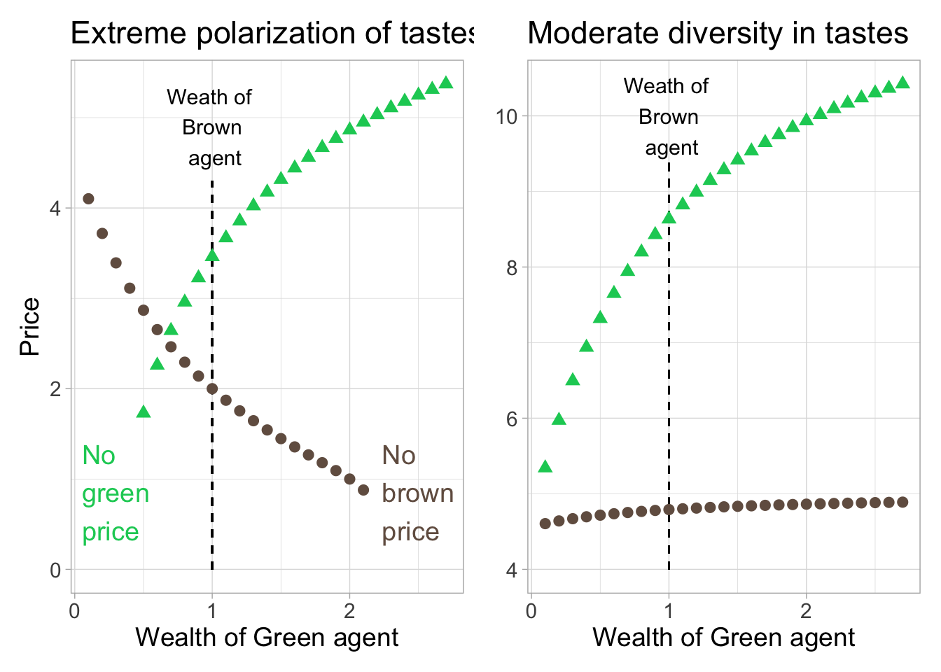
FIGURE 4.1: Theoretical predictions. We plot the price of two assets as a function of the wealth of the Green investor (the wealth of the Brown investor is kept constant at unit value). Prices for the green asset (e=1) are shown with triangles, while those for the brown asset (e=0) are shown with circles. For some values of the x-axis, prices may not be defined in the left plot.
Note that in the left panel, when Green demand is too small (on the left), green prices are not defined. Reversely, when Green demand is too large, brown prices are not valued (right part of the graph). When tastes are less diverse (right panel), these issues vanish.
4.2 SRI improves performance
A large number of published work comes to the conclusion that sustainable investments are more profitable than aggregate benchmarks or even unethical portfolios. In fact, according to the survey Friede, Busch, and Bassen (2015), 90% of papers report a positive relationship between performance and the propensity to tilt portfolios towards ESG stocks. As early as in Klassen and McLaughlin (1996), it is found that environmentally friendly corporate management is rewarded by positive returns. In another seminal article, Gompers, Ishii, and Metrick (2003) show that corporate governance is a strong (positive) driver of returns in the cross-section. Prior to that, Core, Holthausen, and Larcker (1999) also concluded that weak governance is detrimental to financial performance. In a related study, Auer (2016) find that governance-related screens improve performance and that, in fact, firms that have higher ESG ratings earn higher returns.
In another influential series of papers, Edmans (2011), Edmans (2012) reports that portfolios of firms with highly satisfied employees generate significant alpha, though this could stem from prior underperformance (Celiker, Sonaer, et al. (2021)).27 More fundamentally, Mervelskemper and Streit (2017) find that it is always beneficial for firms to communicate on their ESG policies and disclose related reports and indicators. Notably, this motivates employees, who, in turn, are more productive (Burbano (2021), Hedblom, Hickman, and List (2021)).
Many additional contributions underline the benefits that can be extracted when resorting to ESG data in the allocation process, often by selecting those firms with the highest scores. We list a few references in chronological order below in Table 4.1.
| Reference | Notable finding |
|---|---|
| K. M. Cremers and Nair (2005) | A portfolio that is long firms with high level of takeover vulnerability and short firms with low levels of takeover vulnerability generates an annualized abnormal return of 10 to 15% if public pension fund (blockholder) ownership is high. |
| Derwall et al. (2005) | Eco-efficient portfolios (consisting of firms that are more environmentally friendly) generate higher returns compared to non-eco-effficient strategies. |
| Kempf and Osthoff (2007) | Buying high ESG stocks and selling their low ESG counterparts yields annual returns of 8.7% on average. |
| Evans and Peiris (2010) | ESG is positively linked to stock returns, stock valuation and operating performance. |
| Gil-Bazo, Ruiz-Verdú, and Santos (2010) | SRI funds perform better than their conventional counterparts, even after management fees, but the outperformance comes from specialized funds (see also G. Filbeck, Krause, and Reis (2016)). SRI vehicles from general funds underperform. |
| Giroud and Mueller (2011) | “Weak governance firms have lower equity returns, worse operating performance, and lower firm value, but only in noncompetitive industries.” |
| Deng, Kang, and Low (2013) | In M&A deals, high ESG acquirers generate higher returns and have higher success rates. |
| Eccles, Ioannou, and Serafeim (2014) | Highly sustainable firms outperform poorly sustainable firms both in terms of stock market and accounting performance. |
| L. Cai and He (2014) | It takes time for ESG to pay out. The paper reports that profitability comes after 3 years but not before. |
| Matsumura, Prakash, and Vera-Munoz (2014) | On average, on a 2006-2008 panel of 256 firms, for every additional thousand metric tons of carbon emissions, market capitalization decreases by $212,000. |
| Dimson, Karakaş, and Li (2015) | According to the article, firms that commit to successful ESG engagements benefit from positive abnormal returns. |
| Krüger (2015) | Investors respond strongly negatively to negative CSR events, thereby sanctioning bad firms with negative returns. Also, stocks that face severe ESG controversies significantly underperform their benchmarks (Franco (2020)). However, investors may be tempted to overreact to these ESG controversies (B. Cui and Docherty (2020)). |
| Nagy, Kassam, and Lee (2016) | ESG portfolios have superior alpha, compared to a global (MSCI World) benchmark. |
| Verheyden, Eccles, and Feiner (2016) | ESG screens improve risk-adjusted returns. |
| Price and Sun (2017) | CSR is positively rewarded and CSI is penalized, but the effects of CSI last longer. |
| Lending, Minnick, and Schorno (2018) | Sustainable firms with small boards face lower odds of data breaches, which is beneficial for market returns. index{board} |
| Khan (2019) | The authors report: “In the cross-section, forward stock returns increased monotonically across governance and ESG quartiles.” |
| Kumar, Xin, and Zhang (2019) | Firms with higher climate change exposure experience lower subsequent returns. |
| Z. Li et al. (2019) | Best CSR firms earn positive abnormal returns and are more likely to have positive earnings surprises. |
| Awaysheh et al. (2020) | Best-in-class firms (in terms of ESG scores) outperform their industry peers. |
| Ravina and Hentati Kaffel (2020) | The Green-minus-Carbon factor is rewarded in Europe. In addition, it helps explain the cross-section of stocks by augmenting the 5-factor model proposed by Fama and French (2015). |
| Serafeim (2020) | The article shows that to make ESG data profitable, it is useful to resort to public sentiment about firms’ sustainability performance. |
| Madhavan, Sobczyk, and Ang (2021) | The paper analyzes factor loadings of ESG-tilted funds. They show that they are more exposed to the quality and momentum factors and that they also have high alphas. |
| Khajenouri and Schmidt (2020) | The authors compare conventional equity indices with their sustainable screened counterparts. The authors find that green indices outperform with respect to Sharpe ratios. |
| Guest and Nerino (2020) | When a firm experiences a downgrade in governance rank from the Institutional Shareholder Services, negative returns follow. |
| Naffa and Fain (2020) | Nine ESG-tilted portfolios are built on sustainable themes. All of them yielded positive and significant alpha, even after transaction costs. |
| Abate, Basile, and Ferrari (2021) | Mutual funds that invest in high ESG stocks perform better. |
| Wendt et al. (2021) | A portfolio that is long low emission firms and short high emission firms earns an annual alpha of 3.6% (equally-weighted portfolio) or 5.9% (value-weighted portfolio). |
| Chu et al. (2021) | An aggregate ESG index significantly predicts the aggregate market return (with a positive coefficient). |
| J. Xu, Sun, and You (2021) | Firms with high climate change exposure (measured via the Palmer Drought Severity Index) experience lower future profitability |
| Geczy and Guerard (2021) | “Environmental ratings interact with those forecasted returns and produce excess returns both unconditionally and conditionally” and high ESG stocks earn higher returns than low ESG stocks. |
| Havlinova and Kukacka (2021) | “A 1% increase in the ESG Score is associated with an increase in share price between 0.8% and 0.9%” |
| Glossner (2021) | “firms’ past ESG incident rates predict more future incidents, weaker profitability, and lower risk-adjusted stock returns.” |
| R. Chang et al. (2021) | An aggregate ESG index predicts the stock market index positively between 2009 and 2018. |
| Kazdin et al. (2021) | Firms with low carbon intensities have high excess returns and high productivity. |
| Dor, Guan, and Sun (2022) | The ESG premium in US and European equities has been positive in the past decade, after controlling for other factor exposures. |
In an attempt to unify several competing theories, Giese et al. (2019) list three channels through which ESG may positively affect performance: cash flows (ESG firms yield higher dividends), risk (ESG firms have lower tail risk) and valuation (ESG firms, via a lower cost of capital, have an increased value). In a related study, Antoncic et al. (2020) find that it is not necessarily the raw ESG ratings that matter, but also their dynamics. They show that firms that experience ESG momentum (when ESG scores increase) generate positive alpha (similarly, Conen and Hartmann (2019), Shanaev and Ghimire (2021) and Tsai and Wu (2021) show that ESG score revisions matter). Changes in ESG ratings are found to have a significant impact on subsequent returns in Glück, Hübel, and Scholz (2021). The authors conclude that an improvement in the E pillar can be seen (and can act) as a risk mitigating trigger.
Likewise, T. Kim and Kim (2020) report that firms that enhanced their environmental sustainability by adopting cleaner production practices earn significant alpha. On the other end of the spectrum, Gloßner (2021) reports that a portfolio of firms with ESG incidents (e.g., scandals, accidents, etc.) suffers from negative alpha. This may come from analysts downgrading their earning forecasts for these firms (Derrien et al. (2021)). Waddock and Graves (1997) even document a positive feedback loop: positive financial performance fuels ESG behaviors which in turn generate higher profitability (this optimistic finding was however subsequently challenged in the replication study by X. Zhao and Murrell (2016)).
Finally, Bennani et al. (2018) find that ESG has performed well recently. They document that all three pillars yield positive returns for long-short portfolios, but for different reasons: for E, the performance is driven by higher returns of the long leg, while for S and G, it is driven by the poor performance of the short legs.
4.3 SRI does not impact performance
Theoretically, restricting the investment universe should be detrimental to the profitability of screened portfolios (see next subsection). One reason for this is that voluntarily omitting assets may increase the odds of missing fruitful opportunities. In fact, the reverse argument works as well: screening can also participate to exclude assets that will perform badly. All in all, these two effects compete and the aggregate outcome is unclear. Consequently, it is not surprising that many studies contend that SR investing does not really hurt financial performance (while also not improving it).
In a rebuke to Gompers, Ishii, and Metrick (2003), S. A. Johnson, Moorman, and Sorescu (2009) report that screening firms on governance ratings does not yield more profitable portfolios. Similarly, Core, Guay, and Rusticus (2006), Post and Byron (2015) and Amihud, Schmid, and Solomon (2017) do not find any causal relationship between weak governance, gender balanced boards, or staggered boards, and lower market returns. At the aggregate level, the studies of Hamilton, Jo, and Statman (1993), Guerard Jr (1997), Statman (2000), Bauer, Koedijk, and Otten (2005), Bello (2005), Dolvin, Fulkerson, and Krukover (2019), Plagge and Grim (2020), Wee et al. (2020), Curtis, Fisch, and Robertson (2021) (on mutual funds), Sharma et al. (2021) and Milonas, Rompotis, and Moutzouris (2022), as well as the survey Burghof and Gehrung (2021) and the meta analysis of Hornuf, Yüksel, et al. (2022) compare ethical funds to conventional ones and do not find significant differences in performance metrics (notably, average returns, Sharpe ratio and diversification measures). In the same vein, Capelle-Blancard and Petit (2019) report that markets react insignificantly both to positive and negative ESG news.
Furthermore, responsible screening processes in portfolio construction do not deteriorate performance (see Basso and Funari (2014), J. E. Humphrey, Lee, and Shen (2012), J. E. Humphrey and Tan (2014), Blankenberg and Gottschalk (2018), L. Cai, Cooper, and He (2021) and Chava, Kim, and Lee (2021)), but they do not improve it either (Gibson et al. (2020), Pyles (2020) and Görgen, Jacob, and Nerlinger (2021)). Sautner et al. (2021b) report a zero unconditional risk premium associated to climate change risk. In some sectors (e.g., banking), there is no significant link between CSR and CFP (Soana (2011) – though Bătae, Dragomir, and Feleagă (2021) do find some links depending on the components of ESG).
Likewise, market neutral portfolios built on ESG metrics are neither beneficial nor detrimental to profits (Breedt et al. (2019), W. Dai and Meyer-Brauns (2021)), or, equivalently, have insignificant average returns (Kaiser (2020b)). Furthermore, factor models seem to confirm that ESG is not priced (Xiao et al. (2017)), or add no incremental value, compared to traditional factors (Naffa and Fain (2021), Husse and Pippo (2021)). In Bruno, Esakia, and Goltz (2021) acknowledge that the performance of ESG leaders is appealing, unless other traditional asset pricing factors are taken into account. Indeed, the alpha of ESG portfolios disappears when controlling for the size, value, momentum, low volatility, profitability and investment factors. Overall, the meta study C.-S. Kim (2019) confirms that “SRI performance is not different from conventional investments.” Knoll (2002) provides a theoretical argument to explain this lack of impact: the long-run demand curves for the securities of individual firms are not very steep, hence ethical screening does not shift prices much in the long run.
Baron, Harjoto, and Jo (2011) estimate a broad economic model in which firms have to deal with three markets: the financial market that prices their values, the customer market that purchases their products and a market of social pressure that incentivizes them to pursue sustainable policies. They find that CFP is uncorrelated with CSP and negatively correlated with social pressure.
Finally, we single out a few additional studies. The early meta-analysis of Arlow and Gannon (1982) finds little evidence that links social responsiveness to economic performance. A. Ng and Zheng (2018) document that green energy firms have similar performance compared to non-green energy firms, while Halbritter and Dorfleitner (2015) show that high ESG minus low ESG portfolios do not reveal significantly positive returns. Cheung (2011) finds that stocks that are suddenly included or removed from the Dow Jones Sustainability World Index do not experience any particular shift in average return or risk. Via Fama and MacBeth (1973) regressions, Timár et al. (2021) also does not find any significant pricing ability of ESG scores. This is also true when accounting for errors-in-variables (Auer (2021)). We sum up this section with one of the conclusions of Schröder (2004) (p. 130): “socially screened assets seem to have no clear disadvantage concerning their performance compared to conventional assets.”
4.4 SRI is financially detrimental
At the other end of the spectrum, several studies argue that unethical firms tend to experience higher profitability. One such controversial article is that of Fabozzi, Ma, and Oliphant (2008), which shows that sin stocks (belonging to the adult services, alcohol, biotech, defense, gaming and tobacco industries) produce a combined annual return of 19%, outperforming any reasonable benchmark.28 (H. Hong and Kacperczyk (2009) also find outperformance, but to a lesser extent, while Dimson, Marsh, and Staunton (2020b) do confirm superior performance of sin stocks over the long run, since 1900). Likewise, Bolton and Kacperczyk (2021), Bolton and Kacperczyk (2020), Busch et al. (2020) and Santi and Moretti (2021) find that firms with higher total CO\(_2\) emissions (and changes in emissions) earn higher returns. The former authors conclude: “investors are already demanding compensation for their exposure to carbon emission risk.” Nevertheless, Santi and Moretti (2021) also mitigate this result when focusing on regions with low level of worries about climate change. In these regions, the carbon premium disappears.
Similarly, P.-H. Hsu, Li, and Tsou (2021) document that polluting firms experience higher average returns. Moreover, Delmas, Nairn-Birch, and Lim (2015) also report that improving corporate environmental performance reduces short-term financial performance. In the same vein, Trinks and Scholtens (2017) observe that investing in controversial stocks in many cases results in superior risk-adjusted returns.
Conversely, firms that make significant environmental efforts experience lower returns (Fisher-Vanden and Thorburn (2011)), just as do high ESG firms (D. Luo (2022)) and impact firms (Bernal, Hudon, and Ledru (2021)). One explanation is that reducing the carbon footprint or any source of pollution is too costly and outweighs the potential benefits (S. L. Hart and Ahuja (1996)). A second explanation is under-diversification. On the governance side, Bøhren and Staubo (2016) report that firms with mandatory gender parity on their boards experience lower returns (though a broader examination of the literature leads to a more nuanced conclusion, see Post and Byron (2015)).
At the aggregate level, in their study on university endowment funds, Aragon et al. (2020)} find that funds which enforce sustainable policies have greater volatility and the authors attribute underperformance to higher divestment costs and inefficient diversification. Similarly, Anson et al. (2020) find that sustainable funds have, on average, lower alphas compared to unconstrained funds (see also Liang, Sun, and Teo (2022), who show that, nonetheless, ethical hedge funds attract more flows). Bofinger et al. (2021) find that active ESG funds face the risk of lowering their investment skills because of what the authors call the sustainable trap (the push towards ESG increases the risk of mispricing). Similar findings are outlined in Renneboog, Ter Horst, and Zhang (2008b), El Ghoul et al. (2021) and Jeffers, Lyu, and Posenau (2021) (for impact funds), though the underperformance in returns sometimes translates to statistically insignificantly lower Sharpe ratios. Finally, focusing on the debate on mandatory reductions of greenhouse gases in the U.S., A. W. Hsu and Wang (2013) report that markets react positively to negative ESG news at the company level. Conen and Hartmann (2019) document a reverse effect: “markets react to ESG improvements of top ranked firms with negative abnormal returns.”
From an asset pricing perspective, and according to risk factor analysis, investors should be rewarded for the risk they take when investing in stocks that are exposed to ESG externalities. This is one of the theoretical findings of Pastor, Stambaugh, and Taylor (2021b): the capital asset pricing model (CAPM) alpha of stocks should be negatively proportional to their ESG scores. And indeed, X. Chen and Scholtens (2018) argue that both active and passive SRI funds have negative alphas. Empirically, Brammer, Brooks, and Pavelin (2006), D. D. Lee and Faff (2009), Becchetti, Ciciretti, and Dalò (2018), Lioui, Poncet, and Sisto (2018), Lioui (2018b), Lioui (2018a), Ciciretti, Dalò, and Dam (2020), Adriaan Boermans and Galema (2020), Hübel and Scholz (2020), Alessi, Ossola, and Panzica (2020), Alessi, Ossola, and Panzica (2021) and Cakici and Zaremba (2022) all find that the rewarded ESG factors go long irresponsible firms and short responsible ones. The latter documents that a significant part of the premium comes from small firms (which disclose typically less). Similarly, a portfolio, long sin stocks and short non-sin stock earns a monthly return of 1.33% on average (H. A. Luo and Balvers (2017)). In Kanuri (2020), it is found that in the long run, conventional funds outperform ESG funds (in terms of average returns and Sharpe ratio), even though the latter sometimes fare better.
Also, from an optimization standpoint, using screening processes reduces the investment set. By construction, this shifts the efficient frontier towards a smaller enveloppe, which is, by definition, suboptimal – at least in-sample. This implies the opportunity cost of renouncing to potential profitable assets. For a theoretical discussion on this subject, we refer to Pedersen, Fitzgibbons, and Pomorski (2021). In particular, C. E. Chang and Witte (2010) argue that ESG investing shrinks both average returns and Sharpe ratios, compared to unscreened benchmarks.
Finally, in an original contribution, Jørgensen and Plovst (2021) analyze the hedging cost of sustainability. They measure the price of an insurance derivative that would protect an ESG investor against the underperformance of a green fund versus a conventional fund. The authors find that the incurred cost lies between –0.5% and –3% in terms of annual returns.
4.5 It depends
Not surprisingly, SRI does not deliver performance unconditionally, if and when it does. There are in fact many drivers of this performance and the profitability of ESG strategy can depend on several factors, which we list below. The meta-analysis Hang et al. (2018) is a valuable resource on this topic.
4.5.1 Dimensions
First of all, not all dimensions of ESG are equal. Some studies find that governance screens work well (Gompers, Ishii, and Metrick (2003), L. Bebchuk, Cohen, and Ferrell (2009), Auer (2016), Bruder et al. (2019) and L.-E. Lee, Giese, and Nagy (2020), but environmental screens do not (Auer (2016), Alareeni and Hamdan (2020)). Lepetit et al. (2021) document some trends for each pillars between 2014 and 2021 in Europe and the US. Frambo and Kok (2022) study the impact of each pillar on valuation and returns during the COVID 2020 market crash.
In fact, even within ratings, some provisions, or subcategories are more impactful than others (see L. Bebchuk, Cohen, and Ferrell (2009) and Becchetti, Ciciretti, and Dalò (2018)). In a similar vein, Ziegler, Schröder, and Rennings (2007) finds that E is improving returns, while S is deteriorating them. Likewise, Galema, Plantinga, and Scholtens (2008) and Jayachandran, Kalaignanam, and Eilert (2013) show that some ratings can be beneficial (diversity, environment and product), while others cannot. Within each branch of ESG, some component may also prove more relevant than others. Jacobs, Singhal, and Subramanian (2010) find that philanthropic gifts for environmental causes are associated with significant positive market reaction, while it is the opposite for voluntary emission reduction.
Environmental commitments are not all equal: A. King and Lenox (2002) find that prevention leads to financial gain, but not pollution reduction. Based on KLD data, Geczy, Guerard, and Samonov (2019) show that Human Rights, and Diversity criteria contribute to enhancing portfolio returns. A. Filbeck, Filbeck, and Zhao (2019) find that G is beneficial, E is detrimental and S is not impactful. Giese, Nagy, and Lee (2021) find that pillars can matter at different horizons (short for Governance, long for Social and Environmental). Even inside pillars, variables may have mitigating effects. Naranjo Tuesta, Crespo Soler, and Ripoll Feliu (2020) find that different types of policies on different types of emissions have contradicting effects on financial performance. According to Tsai and Wu (2021), enhancing the environmental score leads to higher relative returns in crisis periods.
Moreover, depending on which fields are considered, results differ. Aswani, Raghunandan, and Rajgopal (2021) underline that academics often use the raw values of emissions (in metric tons of CO\(_2\)), while it makes more sense to consider emission intensities, whereby emissions are scaled by some proxy of firm size (e.g., sales) – which may considerably alter conclusions. Furthermore, depending on the industry (see also below), some ESG fields may be considered as financially material (i.e., expected to have an impact on finances), while other are not. The study Grewal, Hauptmann, and Serafeim (2021) shows that materiality is a strong driver of price informativeness.
Beyond pure ESG fields, the propensity of firms to simply disclose ESG related data is also useful in the allocation process (D’Apice, Ferri, and Intonti (2021)). Finally, in De Franco, Nicolle, and Tran (2021), the authors warn that the ESG dimensions are not the only ones in the field. According to them, the sustainable development goals (SDGs) allow to elaborate alternative metrics that capture other facets of sustainability. For an intelligible introduction on SDGs and their relationships with finance, we recommend the overview of Zhan and Santos-Paulino (2021).
4.5.2 Geography
A second important factor is geography. Many articles document contradicting results when switching from one market to another. Often, ESG strategies are shown to perform for one zone (e.g., US, Europe, or Asia), but not all. We refer for instance to Cortez, Silva, and Areal (2012), Von Arx and Ziegler (2014), Post and Byron (2015), Bruder et al. (2019), Cheema-Fox et al. (2019), Matallı́n-Sáez et al. (2019), Franco (2020), Edmans, Li, and Zhang (2020), D. W. Griffin et al. (2021), Amon, Rammerstorfer, and Weinmayer (2021), Murata and Hamori (2021). and Giese, Nagy, and Rauis (2021) In addition, in Chakrabarti and Sen (2020), it is shown that global indices outperform the market, but regional indices do not. In some papers, however, it is shown that there is no link between sustainability and performance, no matter the geographical zone (see Auer and Schuhmacher (2016)). Lastly, there are so many country-specific studies that it is impossible to cite them exhaustively.
Another facet of geography pertains to where ESG incidents may happen and Groen-Xu and Zeume (2021) show that when they occur abroad. Shocks to incidents are negative overall (-0.6%), but less so when they occur outside the country of headquarters (-0.4%). The authors conclude that their is a home bias in shareholder preferences for ESG externalities.
4.5.3 Time-varying link
The third important factor is chronology. Just like all factor tilts in the world, the ESG style has its moments. The perception of ESG has shifted through time. Ioannou and Serafeim (2015) find that analysts’ recommendations used to be pessimistic toward corporate SR policies. Political changes also impact expectations toward green firms and generate shocks to returns (Ramelli et al. (2021)). We refer to Bauer, Koedijk, and Otten (2005), M. L. Barnett and Salomon (2006), Statman (2006), Climent and Soriano (2011), L. A. Bebchuk, Cohen, and Wang (2013), De and Clayman (2015), Belghitar, Clark, and Deshmukh (2017), Ibikunle and Steffen (2017), In, Park, and Monk (2017), Bennani et al. (2018), Mutlu et al. (2018), Ciciretti, Dalò, and Dam (2020), Z. Li et al. (2019), Vojtko and Padysak (2019), Kanuri (2020), Bansal, Wu, and Yaron (2022), Faccini, Matin, and Skiadopoulos (2021), Lepetit et al. (2021) and Tsai and Wu (2021) for contributions that document the time-varying nature of sustainable investments. M. Barnett (2017) reports that the price of climate risk (evaluated via temperatures) is more significant after 1996, compared to the full sample period of 1948-2019. According to Alda and Vicente (2021), returns of SRI funds do not exhibit seasonal patterns.
Several of the aforementioned studies underline that the profitability of SRI was highest in the most recent periods (see Dumitrescu, Jarvinen, and Zakriya (2021) among many others). The hype surrounding ESG investing (and the related demand) may have pushed the prices up. For instance, it is shown in Azar et al. (2021) that the commitment of global asset managers with respect to sustainability is relatively novel and significant. Relatedly, Bansal, Wu, and Yaron (2022) find that SRI performs well in good times, but badly during economic downturns and crises; J. Nofsinger and Varma (2014) come to the opposite conclusion.
Lioui and Tarelli (2021) disentangle time-series and cross-sectional ESG factors. They document a significant time variation in the alpha of both types of factors, conditional on firm characteristics.
The contribution of Pastor, Stambaugh, and Taylor (2021a) points out that the recent outperformance of sustainable firms is entirely due to aggregate concern over the environment. The authors use the Media Climate Change Concerns (MCCC) index of Ardia et al. (2020) and prove that the long-short green factor sees its performance vanish once it has been controlled for shocks in the MCCC index.
We end this subsection by important articles that show that the good performance of ESG stocks in 2019-2021 can be attributed to increased flows. This is the central hypothesis in Beck (2021). In Avramov, Lioui, et al. (2021), the authors argue that the theoretically negative green premium can be offset if the demand for greenness is high. Preference shocks appeared to have pushed realized returns up recently for green assets.
4.5.4 Industry
A fourth dimension is industry. For instance, Herremans, Akathaporn, and McInnes (1993), Russo and Fouts (1997), Semenova and Hassel (2008), Hoepner and Yu (2017a), Giroud and Mueller (2011), Jooh Lee, Pati, and Roh (2011) (oil and gas), Jo and Na (2012), Auer and Schuhmacher (2016), De Haan and Vlahu (2016), M. Feng, Wang, and Kreuze (2017), Bertolotti and Kent (2019), Alessandrini and Jondeau (2020), Torre et al. (2020), Abdi, Li, and Càmara-Turull (2021) and Kuo, Chen, and Meng (2021) (airlines), Giese, Nagy, and Rauis (2021) and Okafor, Adusei, and Adeleye (2021) find that the impact of ESG depends on the sector of firms. In contrast, Statman and Glushkov (2009) argues that for SRI to reach its full potential, it must only rely on ESG ratings and not on industry screening. Giese, Nagy, and Lee (2021) argue that the weighting of ESG pillars should be sector-specific. Typically, industries are not hit uniformly by rising temperature (see Shaw, Evans, and Turner (2021)). For an analysis on the energy sector, we refer to Brzeszczynski et al. (2019).
4.5.5 Ownership
Finally, a fifth mitigating effect is firm ownership. Nekhili et al. (2017) and Abeysekera and Fernando (2020) indicate that family involvement and ownership is also likely to impact the relationship between CSR and financial performance. Brøgger and Kronies (2020) find that the positivity (and significance) of the ESG factor exists within firms that are owned by unconstrained investors (e.g., mutual and hedge funds). Relatedly, Cheema-Fox et al. (2019) find that the performance of portfolios is strongly linked to institutional investor flows.29 \end{itemize}
4.5.6 Nonlinearities
Some researchers (e.g., M. L. Barnett and Salomon (2006), Brammer and Millington (2008), C. Fernando, Sharfman, and Uysal (2010), Harjoto, Jo, and Kim (2017), Gerged, Matthews, and Elheddad (2021) and Bruna et al. (2022)) manage to reconcile seemingly contradicting results by showing that the relationship between CSR and performance (or risk, in Korinth and Lueg (2022)) is not linear: very good and very bad corporations experience abnormal returns, while those in the bulk of the ESG distribution perform differently. Xie et al. (2019) show that the optimal level of disclosure is in the middle of the distribution and very low or very high disclosure leads to lower performance. Fuente, Ortiz, and Velasco (2021) also document an inverted U-shape. Vu, Lehkonen, and Junttila (2022) report a U-shape, but for emerging markets.
More generally, Wong and Zhang (2021) reveal that the nature of shocks to negative ESG news depend on firm characteristics such as firm size, stock liquidity, S&P500 constituency, and corporate reputation status.
The screening intensity and the type of screens seems to play a role as well (Capelle-Blancard and Monjon (2014)), if only because it impacts the diversification of the portfolio (Jin (2020)). Fairhurst and Greene (2020) also document a non-monotonic impact of ESG scores: extreme CSR policies appear to be harmful, at least on the takeover market. Non-linear patterns are moreover documented in S. Huang and Hilary (2018) for governance proxies. Asymmetric preferences of investors (who are indifferent to best-in-class, but penalize worst-in-class firms with negative E and G scores) are revealed in J. R. Nofsinger, Sulaeman, and Varma (2019). One other route to explain diverging results in the field is to argue that models are misspecified, e.g., when important independent variables are omitted (see McWilliams and Siegel (2000)). The way ESG criteria are integrated in the portfolio design can also matter. In their study on the Australian market, Fan and Michalski (2020) find that simple ESG sorts have disappointing performance, but combined with other factors, like quality or momentum, boosts their returns.
The way and reason why firms disclose CSR actions is also likely to matter. Bams, Kroft, and Maas (2021) separate three dimensions in CSR performance and disclosure. First, strategic CSR refers to genuine sustainability for the sake of sustainability. Second, CSR as insurance is a more passive approach to sustainability through which boards and firms “conform to the institutional pressure for CSR by providing a minimal level of CSR to mitigate risks and maintain their licence to operate.” Finally, there is greenwashing. Bams, Kroft, and Maas (2021) find that firms which choose the former outperform the others in both realised social and financial dimensions.
We end this subsection with five references. M. L. Barnett and Salomon (2006) contend that risk-adjusted returns of ESG strategies depend non-linearly in screening intensities. López-Arceiz, Bellostas-Pérezgrueso, and Moneva (2018) argue that the profitability of SR funds is strongly impacted by the cultural environment in which the fund operates. Dorfleitner, Kreuzer, and Sparrer (2020) find that the weighting scheme of portfolios can matter, as well as the size of companies. Assael and Challet (2021) show that ESG attribute help explain, via boosted tree algorithms, the sign of firms’ CAPM alpha. In addition, higher ESG scores are generally associated with larger returns for small firms, but smaller ones for large companies. Finally, Ardia et al. (2020) (following Pastor, Stambaugh, and Taylor (2021b)) find that the profitability of green minus brown portfolios depends on the aggregate concern with respect to climate threats.
4.6 CSR and risk
The question of whether SRI is an efficient way to hedge risk remains open. This has critical implications for institutions such as pension funds (Sautner and Starks (2021)) in the case of downside risk. Becchetti et al. (2015) find that SR funds performed less badly during the 2007-2008 financial crisis, compared to conventional funds. De and Clayman (2015) and Hoepner et al. (2021) document a negative relationship between ESG ratings and risk (measured by stock volatility and downside variance). C. G. Dunbar, Li, and Shi (2021) find that CSR is only a vector of risk reduction if the governance of firms seeks transparency and corporate social performance. In their study on European funds, Gonçalves, Pimentel, and Gaio (2021) reveal that green funds outperform conventional funds in times of crises.
Finally, two rather contrarian articles, Brav and Heaton (2021) and Heaton (2021) suggest that “prudent” investors might want to invest in brown assets in order to hedge against the likelihood that the transition to a greener economy fails to materialize. They highlight the probabilities of scenarii in which brown assets would outperform their green counterparts.
The COVID-19 pandemic yielded a thread of event studies that aim at understanding if sustainability mitigated risk. We list a few such contributions below. Singh (2020) finds that the ESG factor performed well during the COVID-19 market crash (see Mahmoud and Meyer (2021) for an in-depth analysis of the drivers of ESG preferences posterior to this drawdown). Similarly, Pástor and Vorsatz (2020) and Omura, Roca, and Nakai (2020) report that sustainable funds outperformed conventional ones during the market meltdown. Akhtar, Veeraraghavan, and Zolotoy (2021) document a positive effect of gender diversity on the abnormal performance of US stocks during the period between March and April 2020. In Xiong (2021), firms with low ESG risk are found to be outperforming those with high ESG risk. Likewise, in their studes on Indian stocks, Arora, Sur, and Chauhan (2021) and Beloskar and Rao (2022) reveal that sustainable firms fared better than brown ones during the pandemic. Similar results are obtained on European data in Pizzutilo (2021).
However, Folger-Laronde et al. (2020), Demers et al. (2021), Mahmoud and Meyer (2020), Capelle-Blancard, Desroziers, and Zerbib (2021), Chiappini, Vento, and De Palma (2021), Gianfranco Gianfrate, Kievid, and Dijk (2021), Pavlova and Boyrie (2021) and Yousaf, Suleman, and Demirer (2021) see little or no hedging power of ESG-driven funds during the pandemic.30 Glossner et al. (2021) find no evidence that investors shifted toward ESG firms during the COVID-19 crisis and Singh (2021) finds evidence that investors shifted from ESG equities to ESG bonds. Finally, ESG returns may also be contingent on investor sentiment (Azevedo, Kaserer, and MS Campos (2021)).
Below, we list further contributions that conclude that ESG is positively, negatively, or weakly linked to risk.
- ESG reduces risk. CSR engagement reduces risk in controversial industries (Jo and Na (2012)). Social irresponsibility is linked to higher risks (Oikonomou, Brooks, and Pavelin (2012)). Board quality reduces many types of risk (Kaiser (2020a)). Hedge funds can benefit from risk-mitigating properties of ESG investments (Duanmu et al. (2021)). A few articles favorably compare traditional indices to their green counterparts during downturns (Becchetti et al. (2015), Gonçalves, Pimentel, and Gaio (2021), Ouchen (2021)). Other contributions include: McGuire, Sundgren, and Schneeweis (1988), El Ghoul et al. (2011), J. E. Humphrey, Lee, and Shen (2012), Kong et al. (2020) and F. He et al. (2022) (idiosyncratic risk), Harjoto, Jo, and Kim (2017), Bernile, Bhagwat, and Yonker (2018), Monti et al. (2019), Gibson et al. (2020), Lopez de Silanes, McCahery, and Pudschedl (2020), Karwowski and Raulinajtys-Grzybek (2021), Olofsson et al. (2021) and Brodmann, Wuthisatian, and Malladi (2021). ESG also seems negatively related to tail risk (Bax et al. (2021), Xiong (2021)), to stock crash risk (G. Wu and You (2021) find negative correlation with the quality of green patents, but not their quantity; JinCheol Bae, Yang, and Kim (2021) report a negative overall relationship with ESG); J. Feng, Goodell, and Shen (2021) analyze the Chinese market, to default risk (Aslan, Poppe, and Posch (2021), H. Li, Zhang, and Zhao (2022) (in China)) and to bank instability (Chiaramonte et al. (2021)).
- ESG is riskier. R. J. Bianchi et al. (2010) document a negative effect of ESG: green funds have higher betas than conventional funds during recessions. A. C. Ng and Rezaee (2020) find that ESG performance is positively linked to idiosyncratic volatility. Fiordelisi et al. (2021) find that ESG ETFs perform worse than the market during economic downturns. Similar conclusions are obtained by Bansal, Wu, and Yaron (2022).
- Link is not clear. Just like for pure performance, risk is not unequivocally linked to ESG. CSR is weakly linked to risk (Oikonomou, Brooks, and Pavelin (2012)).
- Downside risk. On this topic, we refer to Monti et al. (2019), Shafer and Szado (2020), J. R. Nofsinger, Sulaeman, and Varma (2019) and Richey (2020). The latter shows that sin stocks are defensive in bad times. For a focus on US banks, we recommend the contributions of Tasnia, AlHabshi, and Rosman (2021) and Chaudhry, Saeed, and Ahmed (2021).
-
Implied volatility. Firms that belong to industries with higher ESG-sales dynamism are associated with lower implied volatilities (Patel, Pearce II, and Oghazi (2020)).
- Systemic risk. Better corporate governance in banks helps reducing bank interconnectedness and maintaining financial stability (Aevoae et al. (2022)). Cerqueti et al. (2021) and Cerqueti et al. (2022) find similar mitigating effects of ESG in an exercise of stress scenarios of portfolio litigation.
4.7 ESG and other financial metrics
Beyond pure stock-market profitability, ESG seems to be favorably related to the metrics listed in Table 4.2. With respect to valuation and cost of equity, let us briefly recall that, according to Gordon’s dividend model, the firm value is equal to \(V_0/(c-g)\), where \(c\) is the cost of capital (e.g., weighted average cost of capital (WACC)) and \(g\) is the growth rate of cash flows (or dividends). ESG issues can impact both channels. Firm value can increase if \(g\) increases, or if \(c\) decreases, e.g., because investors perceive lower risk. Derrien et al. (2021) show that with respect to ESG incidents, it is the first channel that matters most.
4.8 Empirical illustration
We close this chapter with a small empirical exercise. We compare two US equity indices: one conventional, and one ESG-based. The conventional index is the S&P 500, arguably the reference yardstick for US equities, both among practitioners and scholars alike. The ESG portfolio is the iShares MSCI USA ESG Select ETF, which performs sustainability screens that are based on sectors, as well as on ESG scores. In December 2020, the index comprised 202 stocks, which makes it less diversified, compared to the S&P 500.31 The series start on January 28\(^{th}\), 2005, which is the inception date of the ESG index. It is notoriously complicated to find reliable ESG data prior to 2005. In Figure 4.2, we plot the time-series of the two indices.
library(quantmod)                             # Package for financial data retrieval
library(lubridate)                            # Package for date management
tickers = c("SUSA", "SPY")                    # Ticker names
prices <- getSymbols(tickers, src = 'yahoo',  # Yahoo source
                     from = "2005-01-28",
                     to = Sys.Date(),
                     auto.assign = TRUE,
                     warnings = FALSE) %>%
    map(~Ad(get(.))) %>%
    reduce(merge)

norm_ <- function(v){return(v/v[1])}
prices <- apply(prices, 2, norm_)
prices <- tibble(date = as.Date(rownames(prices)), as_tibble(prices))
colnames(prices)[2:3]<-c("MSCI_ESG", "SP500")
prices %>%
    pivot_longer(-date, names_to = "Index", values_to = "Value") %>%
    ggplot(aes(x = date, y = Value, color = Index)) + geom_line() + theme_light() +
    scale_color_manual(values = c("#0DCD64",  "#0D70CD"), labels = c("MSCI ESG", "S&P 500")) +
    theme(legend.position = c(0.2, 0.8)) + xlab("Date") + ylab("Index Value") +
theme(text = element_text(size = 16)) 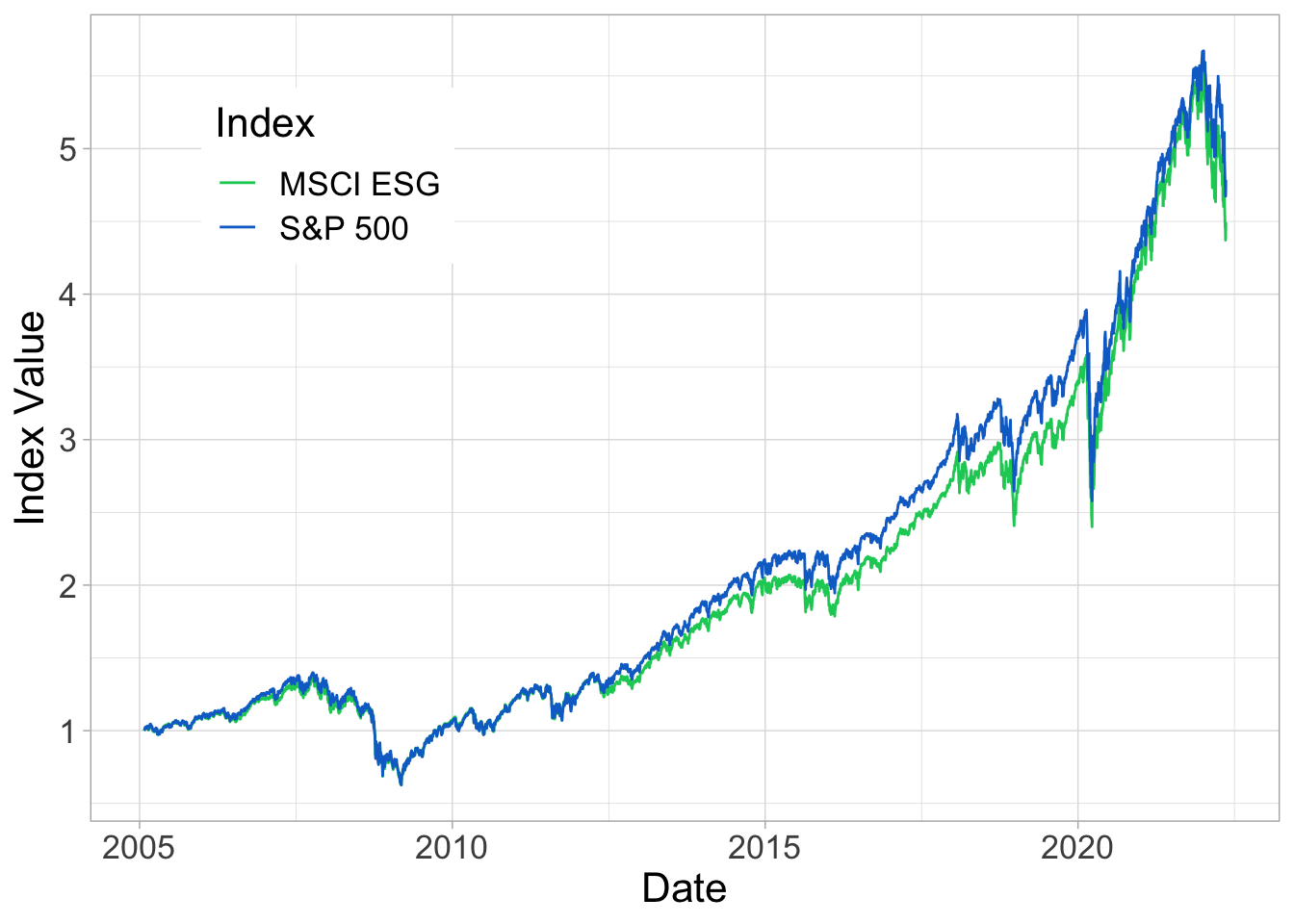
FIGURE 4.2: Performance comparison. We plot the index values (S&P 500 and iShares MSCI USA ESG Select ETF), onward from January 28th, 2005 (inception date of the ESG portfolio). The series are normalized so that their initial value is one.
At first sight, the first-order conclusion is that there is not much difference between the two series. In the first half of the sample, the lines are hardly distinguishable. Between 2012 and 2019, the S&P 500 seems to outperform marginally, but 2020 has eroded part of this superiority (see below). In Table 4.3, we compute a few performance metrics.
library(tseries)
library(kableExtra)
returns <- prices %>%                                                      # returns
    mutate(MSCI_ESG = MSCI_ESG/lag(MSCI_ESG) - 1,
           SP500 = SP500/lag(SP500) - 1) %>%
    na.omit()

prices <- prices %>% na.omit()                                             # remove missing points
ret <- (prices[nrow(prices), 2:3] / prices[1, 2:3]) ^ (252/nrow(prices))-1 # returns
vol <- apply(returns[,2:3], 2, sd) * sqrt(252)                             # volatility
ratio <- ret/vol                                                           # Sharpe ratio (proxy)
mdd <- apply(prices[,2:3] %>% na.omit(), 2, maxdrawdown)                   # max drawdown
var5 <- apply(returns[,2:3], 2, function(v) quantile(v, probs = 0.05))     # Value-at-Risk

tibble(Index = c("MSCI ESG", "S&P 500"),
       Return = as.numeric(ret),
       Volatility = vol,
       Ratio  = as.numeric(ratio),
       MaxDrawdown = as.numeric(c((prices[mdd$MSCI_ESG$to,2]-prices[mdd$MSCI_ESG$from,2])/prices[mdd$MSCI_ESG$from,2],
                       (prices[mdd$SP500$to,3]-prices[mdd$SP500$from,3])/prices[mdd$SP500$from,3])),
       ValueatRisk = var5) %>%
kableExtra::kable(caption = 'Performance indicators.')| Index | Return | Volatility | Ratio | MaxDrawdown | ValueatRisk |
|---|---|---|---|---|---|
| MSCI ESG | 0.0868963 | 0.1864341 | 0.4660966 | -0.2637472 | -0.0175106 |
| S&P 500 | 0.0915205 | 0.1951129 | 0.4690642 | -0.3371726 | -0.0181815 |
All values are arguably close, and no difference in any metric would pass a test of statistical significance. The broad market index has a marginal superiority in returns, but it is bested across both risk measures. The volatility-adjusted average return is even slightly higher for the ESG index. Overall these results are most in line with those of Section 4.3: in the long run, its is hard to find evidence (in this small sample) of outperformance in one way or the other.
Researchers and practitioners often seek to determine if ESG exposure acts as a hedge in bad times. To shed some light on this question, we zoom in on two sub-periods of the sample, namely the years 2008–2009, and 2020. These are shown in Figure 4.3, where the series are scaled to start at unit value.
g2 <- prices %>%
    filter(date > "2019-12-31", date < "2021-06-30") %>%
    mutate(across(.cols = c(2,3), norm_)) %>%
    pivot_longer(-date, names_to = "Index", values_to = "Value") %>%
    ggplot(aes(x = date, y = Value, color = Index)) + geom_line() + theme_light() +
    scale_color_manual(values = c("#0DCD64",  "#0D70CD"), labels = c("MSCI ESG", "S&P 500")) +
    theme(legend.position = c(0.75, 0.2)) + xlab("Date") + ylab(element_blank()) +
    theme(text = element_text(size = 14), aspect.ratio = 0.8)

g1 <-prices %>%
    filter(date > "2007-12-31", date < "2010-01-01") %>%
    mutate(across(.cols = c(2,3), norm_)) %>%
    pivot_longer(-date, names_to = "Index", values_to = "Value") %>%
    ggplot(aes(x = date, y = Value, color = Index)) + geom_line() + theme_light() +
    scale_color_manual(values = c("#0DCD64",  "#0D70CD"), labels = c("MSCI ESG", "S&P 500")) +
    theme(legend.position = c(0.65, 0.8)) + xlab("Date") + ylab(element_blank()) +
    theme(text = element_text(size = 14), aspect.ratio = 0.8)
g1 + g2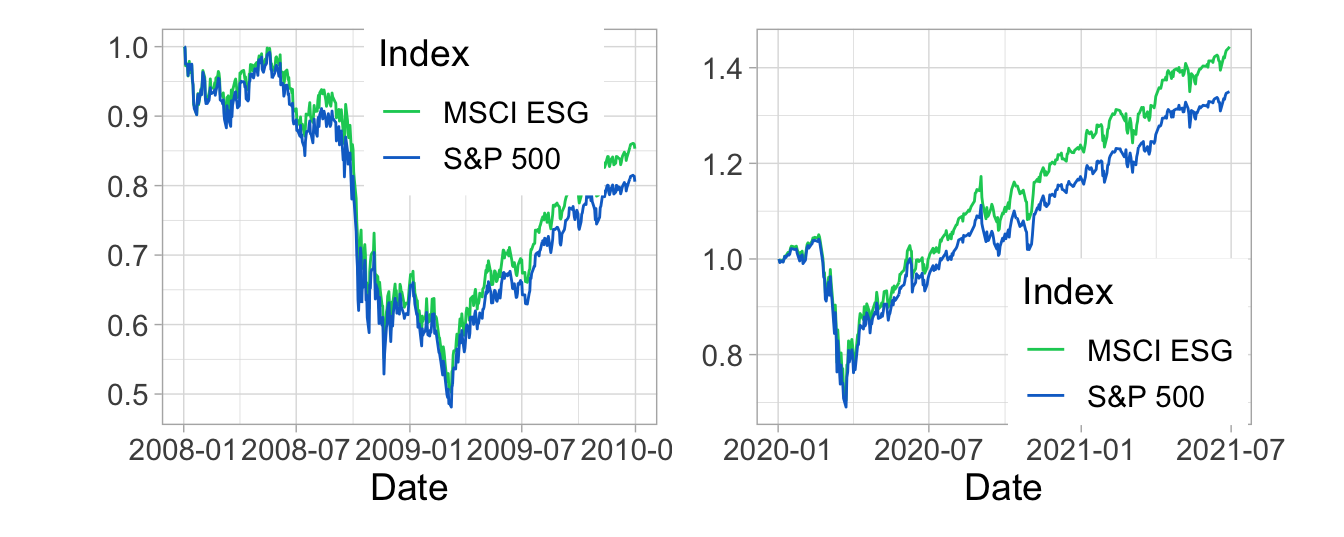
FIGURE 4.3: Focus on 2008–2009 and 2020–2021. We plot the index values, from January 1st, 2008 to December 31st, 2009 (left panel) and from January 1st, 2020 to the end of June 2021 (right panel). The series are normalized so that their initial value is 1
In 2020 (right panel), the two curves move closely together until April, which means that the sustainable tilt did not immunize the ESG portfolio against the crash.32 To a certain extent, this is also true for the subprime crisis in 2008.
However, the interesting pattern is probably revealed after the crises. It is in the aftermath of the crashes that differences materialize, to the benefit of the ESG index. It is as if, after being burnt by an extreme event, investors redirect flows toward more sustainable assets. This is consistent with some conclusions of Dyck et al. (2019). Nevertheless, zooming out back to Figure 4.2 reveals that this effect fades. After 2009, the S&P 500 out-performed until 2019 (see Figure 4.3), as if the appeal of ESG stocks decreases with the time span after a crash.
g2 <- returns %>%
    mutate(year = year(date)) %>%
    pivot_longer(-c(date, year), names_to = "Index", values_to = "return") %>%
    group_by(year, Index) %>%
    summarise(avg_return = mean(return)*252) %>%
    ggplot(aes(x = year, y = avg_return, fill = Index)) + geom_col(position = "dodge")  + theme_light() +
    scale_fill_manual(values = c("#0DCD64",  "#0D70CD"), labels = c("MSCI ESG", "S&P 500")) +
    theme(legend.position = c(0.45, 0.2)) + xlab(element_blank()) + ylab("Annualized Return") +
    theme(text = element_text(size = 14))
g1 <- returns %>%
    mutate(year = year(date),
           diff = MSCI_ESG-SP500) %>%
    select(year, diff) %>%
    group_by(year) %>%
    summarise(avg_return = mean(diff)*252) %>%
    ggplot(aes(x = year, y = avg_return)) + geom_col()  + theme_light() + xlab(element_blank()) +
    ylab("ESG - S&P") + theme(text = element_text(size = 14))

g2 + g1 + plot_layout(heights = c(2, 1))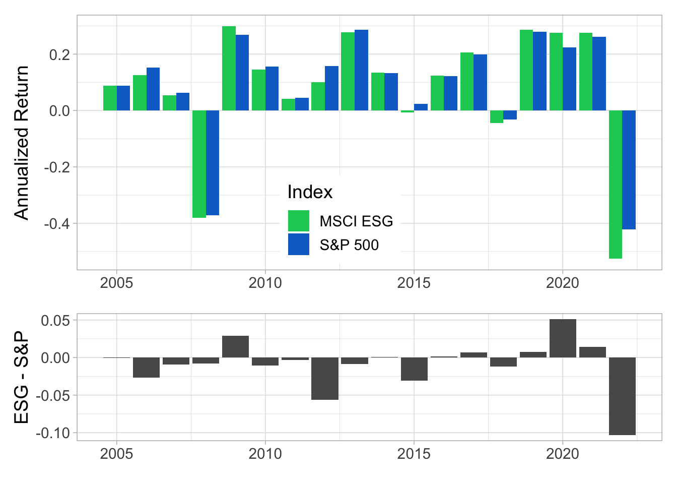
FIGURE 4.4: Annual returns. In the upper panel, we plot the average daily returns multiplied by 252, on a year-by-year basis. The lower panel shows the difference between the two indices (MSCI ESG minus S&P 500).
To illustrate the shifting relative risk of ESG portfolios, we compute the volatility ratio between the S&P 500 and the ESG index in Figure 4.5. Realized volatilities are computed as the standard deviation of the daily returns over the past 60 trading days. While the S&P 500 is more often the most volatile index, the ESG portfolio does run through some pockets of superior risk, especially between 2016 and 2019.
library(RcppRoll)
vol <- returns %>%
    mutate(MSCI_ESG = roll_sd(MSCI_ESG, 60, fill = NA),
           SP500 = roll_sd(SP500, 60, fill = NA),
           vol_ratio = SP500/MSCI_ESG,
           col = vol_ratio > 1,
           vol_SP = if_else(col, vol_ratio, as.numeric(NA)),
           vol_MS = if_else(!col, vol_ratio, as.numeric(NA))) %>%
    pivot_longer(c(vol_SP, vol_MS), names_to = "Index", values_to = "vol")
vol %>% ggplot() +
    geom_line(aes(x = date, y = vol, color = Index), show.legend = FALSE) + theme_light() +
    theme(text = element_text(size = 14)) +
    geom_hline(yintercept = 1, linetype = "twodash", size = 1.4) + xlab(element_blank()) +
    ylab("Volatility ratio (SP500/ESG)") + scale_color_manual(values = c("#0DCD64",  "#0D70CD")) +
    annotate(geom = "text", x = as.Date("2012-01-01"), y = 0.85, label=TeX("MSCI ESG more volatile"), color="#0DCD64", size = 5) +
    annotate(geom = "text", x = as.Date("2014-01-01"), y = 1.25, label=TeX("S&P 500 more volatile"), color="#0D70CD", size = 5)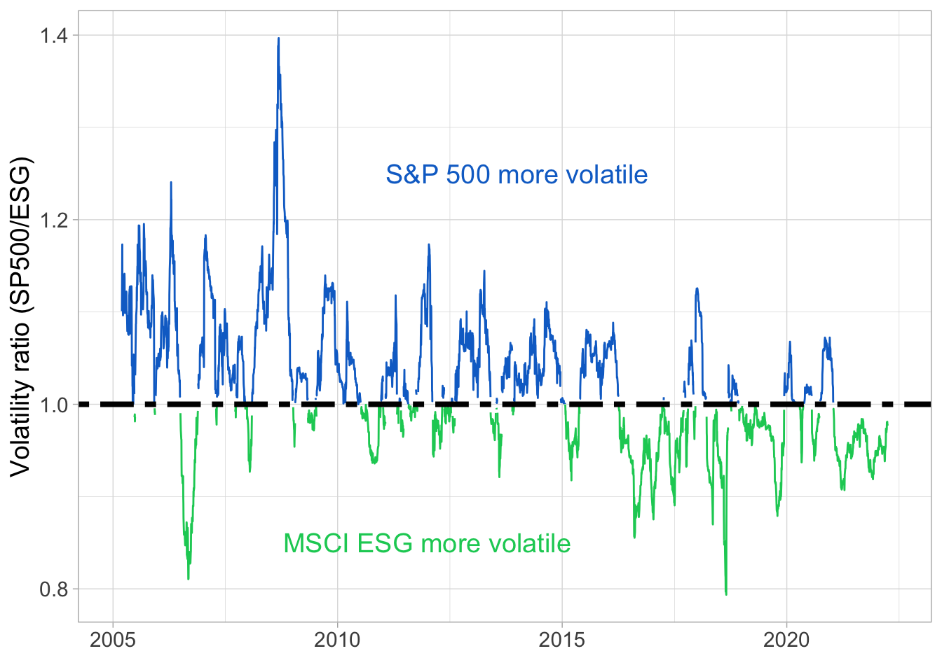
FIGURE 4.5: Volatility ratio. We plot the ratio of the S&P 500 volatility divided by the volatility of the MSCI ESG index. Realized volatilities are computed as the standard deviation of the daily returns over the past 60 trading days.