6 Climate change risk

“Climate risk is investment risk” (Scanlan (2021)).

This chapter is dedicated to the perils of global warming and their impact on firms and on the financial market in general.³⁵ The importance of this threat has long been mostly overlooked but is now even documented by governmental commissions in the US (see Behnam et al. (2020)). In fact, as early as the mid-1990s, Porter and Van der Linde (1995) called for a change of paradigm in the trade-off between environmental friendliness and competitiveness. At the time, the authors based their arguments on the need to incorporate innovation (and its dynamics) as a key variable. Nowadays, this trade-off seems more focused on long-term risks related to climate change (see, e.g., Daniel, Litterman, and Wagner (2018), M. Barnett, Brock, and Hansen (2020)).

We start this chapter by simply quoting the provocative paper of Mayer (2019): “natural capital is very different from other forms of capital and arguably should not be viewed as a capital at all. Its distinctive features are its renewable and restorative properties, its irreversibility, its living and evolving nature, and the fact that it was inherited, not created, by humans.” Climate risks are now documented and for instance surveyed in Breitenstein, Nguyen, and Walther (2021) and Giglio, Kelly, and Stroebel (2021). Luckily, international cooperation on the matter seems to be intensifying (Carattini et al. (2021))!

Nevertheless, in their survey of experts, Stroebel and Wurgler (2021) find that the latter overwhelmingly believe that asset prices underestimate climate risks. According to them, the short term risk is regulatory (e.g., benefits being curtailed by carbon taxes), while the long term risk is physical (e.g., natural disasters impacting production, transport, or consumption of goods). The regulatory risk, combined to risks related to shifts in consumer preferences for instance are aggregated into what are often referred to as transition risks. These risk are tantamount for some sectors (e.g., fossil fuels), and the likelihood of stranded assets is for instance discussed in Cahen-Fourot et al. (2021). The authors use input-output matrice to derive industry and country stranding multipliers. Counter-intuitively, the countries that are the most at risk are France, Australia and Slovakia, while those the least at risk are the USA, Italy and China. We refer to Apel, Betzer, and Scherer (2021) for a high frequency stock-specific analysis of transition risks.

This chapter is divided in four separate parts. The first part deals with discounting utility and cash flows in uncertain environments. The second part covers measurement issues in the assessment of climate change. The third part gives a quick overview of some macro-economic impacts of global warming. Finally, the last subsection demonstrates that investors increasingly care about these issues (which echoes Section 3.1).

6.1 Uncertain discounting

The mathematics-averse reader is advised to skip this subsection.

Discounting is a central topic in financial analysis because it translates the value of future flows into current units. Depending on preference and beliefs, discounting factors will alter expected cash flows and utility. In this subsection, we briefly recall how uncertainty may affect returns. We start by recalling the model of Ramsey (1928).

An entity (individual or society) seeks to optimize a definition of global welfare

\[\begin{equation} W=\sum_{t=0}^\infty \beta^tu(c_t), \label{eq:ramsey0} \end{equation}\] where $u(\cdot)$ is some utility function, $c_t$ is time-$t$ consumption, and $\beta \in (0,1)$ is the discounting intensity. A low beta signals a strong preference for the most imminent dates, while a high beta puts a higher weight on the distant future. Sometimes, the conventions $\beta=(1+\rho)^{-1}$ and $\beta=e^{-\delta}$ are used, in which case $\rho$ and $\delta$ are the discount rates. The entity

has capital wealth $k_t$ which it can invest on a financial asset,
earns a wage $w_t>0$, and
faces a budget constraint:³⁶ \[\begin{equation} k_{t+1} = e^{r_t}k_t + w_t-c_t \ge 0, \tag{6.1} \end{equation}\] that is, future wealth equals wealth invested on the asset at (log-)rate $r_t$, plus wage, minus consumption. It is naturally assumed that the wealth remains positive.

The entity must choose the levels of investment $k_t$ and consumption $c_t$ to maximize the welfare $W$. Taking into consideration two consecutive points in time, the (restricted) Lagrangian reads \[\begin{align} \mathcal{L}= \ &\beta^t u(c_t) - \lambda_t(k_{t+1} - e^{r_t}k_t - w_t+c_t ) &(\text{time }t )\\ &+\beta^{t+1} u(c_{t+1}) - \lambda_{t+1}(k_{t+2} -e^{r_{t+1}}k_{t+1} - w_{t+1}+c_{t+1} ), &(\text{time }t+1 ) \nonumber \label{eq:L} \end{align}\] and the first-order conditions command \[\begin{equation} \frac{\partial \mathcal{L}}{\partial c_t} = \beta^tu'(c_t)-\lambda_t=0, \quad \text{and }\quad \frac{\partial \mathcal{L}}{\partial k_{t+1}}= -\lambda_t+\lambda_{t+1}e^{r_{t+1}}, \tag{6.2} \end{equation}\] and plugging the left part into the right one, this translates to \[\begin{equation} \beta^tu'(c_t)= \beta^{t+1}u'(c_{t+1})e^{r_{t+1}} \Longleftrightarrow \frac{u'(c_t)}{u'(c_{t+1})}=\beta e^{r_{t+1}}. \tag{6.3} \end{equation}\] This equation is a cornerstone of consumption-based asset pricing (see Cochrane (2009)) because it links returns to the ratio of marginal utilities (present versus future). While the asset pricing literature usually takes the route of the pricing kernel (or stochastic discount factor), we pursue the analysis as it is derived in economics.

Often, the utility function is chosen to be CRRA, so that $u(x)=x^{1-\alpha}/(1-\alpha)$, for $\alpha$ strictly positive but not equal to one (in the latter case, the logarithmic function is used instead). In this case, with $\beta=e^{-\delta}$, and \[\begin{equation} \left( \frac{c_t}{c_{t+1}}\right)^{-\alpha}= e^{r_{t+1}-\delta} \Longleftrightarrow r_{t+1}=\delta +\alpha \log \left(\frac{c_{t+1}}{c_t} \right). \tag{6.4} \end{equation}\] The above rate $r_{t+1}$ is sometimes referred to as the social discounting rate (SDR) in the public economics literature. It is such that the entity is indifferent between the two options: - consume more at time $t$ and enjoy immediate utility or
- reduce consumption and invest to gain more at time $t+1$, with a discount of $\delta$.

Another way to interpret the result is that the return on investment on the left-hand side in Equation (6.4) must be equal to the welfare-preserving inter-temporal trade-off on the consumption (right-hand side). If consumption growth increases, then the SDR should also increase, in order to cover the future consumption needs. The SDR is very important because it is a crucial component in the computation of the social cost of carbon (see Anthoff, Tol, and Yohe (2009) and Section 7.2). It is used to discount (in time) the welfare of a population, often by attenuating the importance of aggregate utility (based on consumption) as time passes.

One interesting extension of this model pertains to the alteration of this social discount rate when consumption growth is random.³⁷ This idea has gained traction at least since Gollier (2002), and they are applied to a climate change paradigm in Gollier (2013)).³⁸ Let us assume that $g_{t+1}=\log(c_{t+1}/c_t)$ is Gaussian with mean $\mu$ and variance $\sigma^2$. Under CRRA preferences, at time $t$, we can take the expectation of Equation (6.3) as follows: \[\begin{equation} e^{\delta-r_{t+1}}=\mathbb{E}[e^{-\alpha g_{t+1}} ] \Longrightarrow r_{t+1}=\delta +\alpha \mu-\alpha^2 \frac{\sigma^2}{2}, \tag{6.5} \end{equation}\] which means that uncertainty in future consumption decreases the return. Straightforwardly, any investor prefers less risk. For the interested reader, we recommend a few additional references on the topic of climate economics: Ackerman et al. (2009), Heal (2009), Weitzman (2009), and, more recently, Gollier (2021) on the topic of carbon prices. For a recent discussion on estimation issues, we point to Newell, Pizer, and Prest (2021).

Lastly, on a related issue, Gelrud (2021) produces a theoretical model aimed at quantifying the rate at which climate change mitigation project should be discounted. The authors shows that this rate should be smaller than the risk free rate - and that it is optimal to invest in such projects as fast as possible.

6.2 Measurement issues

In order to quantify the risk of global warming, it is first imperative to define which variables drive the externalities. They can be direct measurements of the underlying phenomenon (e.g., local or aggregate temperatures and rainfall), or time-series of potential drivers thereof (greenhouse gas (GHG) and carbon dioxide (CO$_2$) emissions). In addition to measuring, it is also useful to predict or even nowcast such quantities: see Bennedsen, Hillebrand, and Koopman (2021) for a methodology on CO$_2$ emissions. Prediction models are important because they seem to drive market participants’ expectations (Schlenker and Taylor (2021)). International groups, such as the Intergovernmental Panel on Climate Change (IPCC) periodically disclose in-depth studies that contain numerous estimates on past, present and future indicators (emissions, temperatures, precipitations). On the topic of climate data, we also refer to Tankov and Tantet (2019) for a very enlightening discussion on the dimensions and stakes for financial agents.

Measuring and reporting climate-related indicators requires resources, which is why it is often performed by national or international research centers. Per se, the equipment (thermometers, CO$_2$ sensors, etc.) are not particularly expensive. It is keeping track of trustworthy measurements over long time ranges which is costly. With regard to the evolution of CO$_2$, one benchmark is the measurement by the US Earth System Research Laboratories near the summit of the Mauna Loa volcano.³⁹ The corresponding time-series is shown in the top panel of Figure 6.1 and shows an indisputable trend.

link <- "ftp://aftp.cmdl.noaa.gov/products/trends/co2/co2_mm_mlo.txt"  # Link for C02 data
co2 <- read.table(link)                                  # Read data
co2 <- co2[,c(1,2,4)]                                    # Keep relevant columns
colnames(co2) <- c("Year", "Month", "CO2_concentration") # Rename columns
# link for temperature anomalies
link <- "https://www.ncdc.noaa.gov/cag/global/time-series/globe/land_ocean/1/9/1880-2021/data.csv"
anomaly <- read_csv(link, skip = 4)                      # Read data

g1 <- co2 %>%
    mutate(date = make_date(year = Year, month = Month, day = 15)) %>%
    ggplot(aes(x = date, y = CO2_concentration)) + 
    scale_x_date(limits = c(as.Date("1880-01-01"), as.Date("2021-06-30"))) +
    geom_line() + geom_smooth(color = "red") + 
    theme_minimal() + theme(axis.title.x = element_blank()) + 
    ylab("CO2 concentration (ppm)") + 
    annotate("text", label = "Data not available", x = as.Date("1920-01-01"), y = 320)
    

g2 <- anomaly %>% 
    ggplot(aes(x = Year, y = Value)) +
    geom_line() + geom_smooth() + theme_minimal() +
    theme(axis.title.x = element_blank()) + 
    ylab("Temperature anomaly")
    
g1 / g2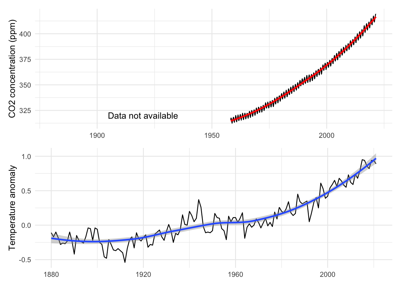

Sample of climate related time-series. We plot atmospheric CO$_2$ levels along with global temperature trends over the period 1960–2021. The data was gathered from the National Oceanic and Atmospheric Administration (NOAA) website.

FIGURE 6.1: Sample of climate related time-series. We plot atmospheric CO$_2$ levels along with global temperature trends over the period 1960–2021. The data was gathered from the National Oceanic and Atmospheric Administration (NOAA) website.

Recent initiatives propose measures at a more granular (i.e., local) level, see for instance Z. Liu et al. (2020) and Dou et al. (2021) as well as the website https://carbonmonitor.org, as well as http://www.climateestimate.net. The latter proposes code snippets in R, Python and MATLAB. This allows to track emissions at the country and sector level and we provide a sample of trajectories for 2019-2021 in Figure 6.2. Clearly, the reduction in emissions appears in China (which was hit earlier) a few weeks before Europe and the US for aviation and ground transport. For industry and power, the impact is more pronounced for China, but the rebound is also marked.

url = 'https://raw.githubusercontent.com/shokru/esgperspectives.github.io/main/data/carbonmonitor.csv'
carbon <- read.csv(url)
colnames(carbon) <- c("zone", "date", "sector", "MtCO2", "timestamp")
carbon <- carbon %>% mutate(date = as.Date(date, format = "%d/%m/%Y"))
carbon %>%
    filter(zone %in% c("US", "China", "EU27 & UK")) %>%
    mutate(month = month(date), year = year(date)) %>%
    group_by(zone, sector, month, year) %>%
    mutate(avg_CO2 = sum(MtCO2, na.rm=T)) %>%
    ggplot(aes(x = date, y = avg_CO2, color = zone, linetype = zone)) + 
    geom_line() +
    geom_vline(xintercept = as.numeric(as.Date("2020-01-13")), linetype = 2, size = 1.2) +
    geom_line() + theme_light() +
    facet_wrap(vars(sector), ncol = 2, scales = "free") + ylab("Monthly CO2 metric tons per capita") +
    xlab("")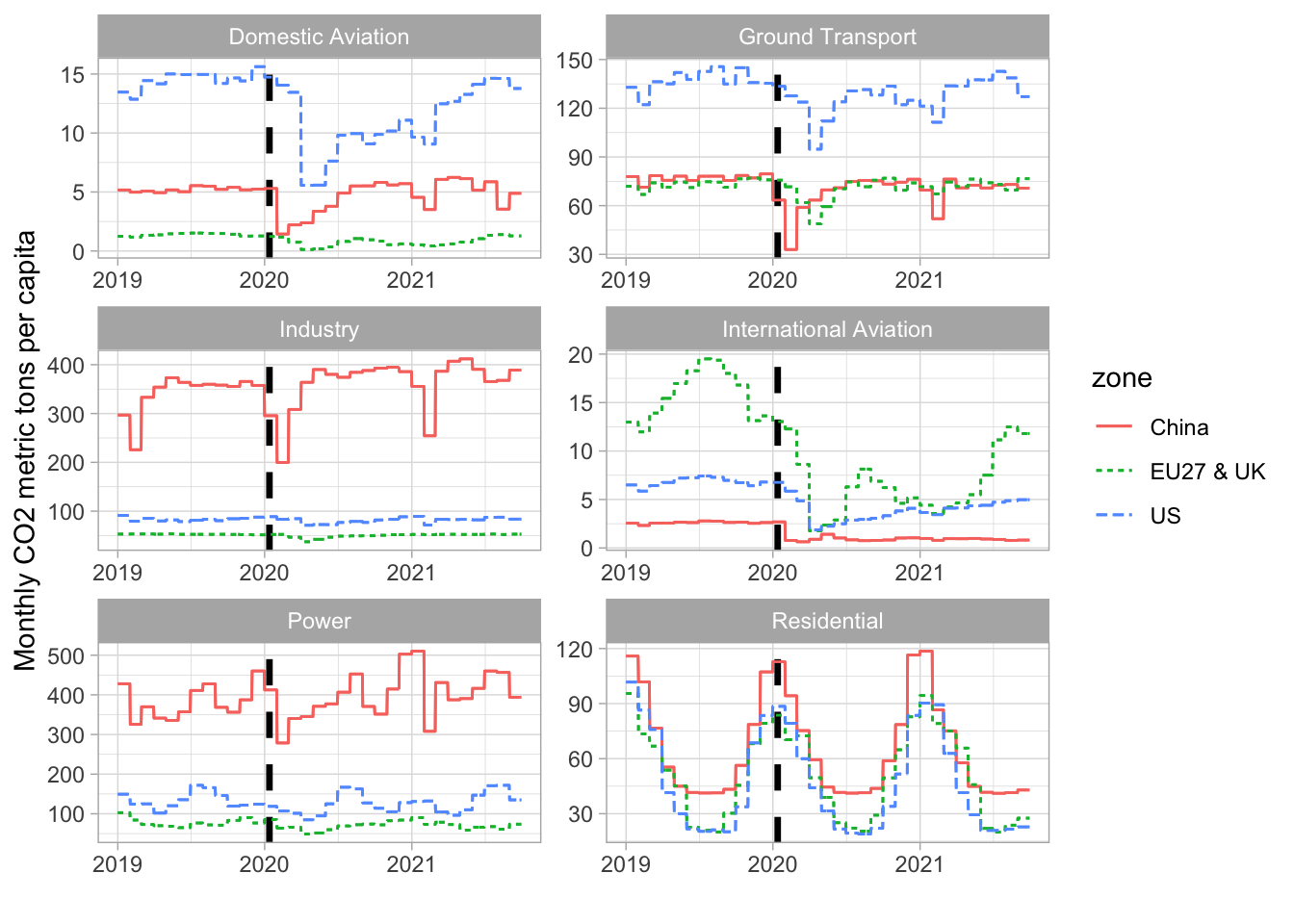

CO2 in the time of COVID-19. We plot the geographic and sector specific estimates for CO$_2$ emissions provided by https://carbonmonitor.org. The vertical dashed line marks January 13th, 2020, which is the date when a first case of COVID-19 was discovered outside China (in Thailand).

FIGURE 6.2: CO2 in the time of COVID-19. We plot the geographic and sector specific estimates for CO$_2$ emissions provided by https://carbonmonitor.org. The vertical dashed line marks January 13th, 2020, which is the date when a first case of COVID-19 was discovered outside China (in Thailand).

At the firm level, we refer to https://climatechangelab.info. The evaluation of climate change exposure is postponed to section 6.4.

For temperatures, the challenge is different because of the dimension of the reporting. Thousands of thermometers track variations in meteorological stations and it is cumbersome to access and aggregate such data. Most sensors are located on land, which only covers 29% of the globe’s surfaces. Thus ocean temperature must also be measured (at their surfaces), and this is performed with ships. We refer to the paper by J. Hansen et al. (2010) for a precise account on this matter. In the lower panel of Figure 6.1, we plot the evolution of the global temperature of our planet. While the curve is less regularly increasing, the trend is again undeniable. The parallel display of the two series reveals a strong correlation. It is now widely accepted that the relationship is causal, whereby CO$_2$ emissions are a key driver of the increase in temperature. We point to Le Treut (2007) for a historical perspective on this debate. More recent contributions document feedback effects (Van Nes et al. (2015)), or clear direct causality (Stips et al. (2016)).

From an investment standpoint, being able to quantify physical risks linked to climate change is important. Hain, Kölbel, and Leippold (2021) show that, just like for traditional ESG metrics, ratings of physical risks are very much provider-dependent. They compare series from Trucost, Carbone 4 Finance, Southpole, Truevalue Labs, and two academic-based measures and find that correlations within sectors are relatively small. This implies that portfolios sorted on these metrics have limited overlaps when switching from one provider to another.

6.3 Stress tests and other measures

In Battiston et al. (2017), GHG emission data is used to stress-test the financial system. In Reinders, Schoenmaker, and Van Dijk (2020), the focus of the stress test study is set on taxes and their impacts. The risk for firms is that governments will be increasingly inclined to penalize polluters, thereby threatening parts of their balance sheets. In their proposal for an integrated stress-testing methodology, Allen et al. (2020) promote a scenario-driven approach in which climate models are intertwined with macro-economic models. The procedure is able to generate individual firms’ probabilities of defaults, as well as market valuations. A similar framework is adopted by Fang, Tan, and Wirjanto (2019), and subsequently combined to mean-variance optimization to build portfolios that are less sensitive to climate change risk. Relatedly, Monasterolo (2020) proposes new climate risk metrics, such as the climate Value-at-Risk, which is computed on corporations that would be most affected in stress scenarios.

In their attempt to measure climate change risk for corporations, Q. Li et al. (2020) proceed very differently: they extract textual sentiment from earning call transcripts. The authors use a dedicated climate-centric lexicon combined to manual verifications. From this, they synthesize several climate risk measures which they study in detail. Chou and Kimbrough (2019) automate the textual screening of firms’ SEC filings. They show that the frequency at which climate change terms are mentioned increases through time, though the patterns differ from one industry to the other. Faccini, Matin, and Skiadopoulos (2021) also analyze textual factors and split risks in two categories: transition risk (via policy (e.g., fiscal) or shifts in consumer preferences) and physical risk (e.g., catastrophes). They find that only the first one is priced in the US stock market.

A. W. Hsu and Wang (2013) also resort to sentiment analysis, but focused on one media outlet (The Wall Street Journal). They measure the negativity of the tone related to climate change articles in the press. Surprisingly, they report that the aggregate market reacts positively to negative news. Natural language processing (NLP) is also exploited in Engle et al. (2020) to build portfolios that hedge investors against negative news related to climate change. In a similar vein, Sautner et al. (2021a) use transcripts of earnings conference calls to assess the exposure of 10,000 firms to opportunity, physical, and regulatory shocks associated with global warming. They use their methodology in a follow-up paper that links climate risk exposure to risk premia. In a different setting, Heo (2021) also uses their data to reveal that firms that are more exposed to climate change risk increase their cash holdings, probably in anticipation of adverse situations. Relatedly, Santi (2021) crafts a climate sentiment index and shows how it dynamically affects the performance of an Emission-minus-Clean portfolio.

For a more computer science-focused perspective on NLP-driven classification of ESG topics and climate risks, we refer to Nugent, Stelea, and Leidner (2020), Raman, Bang, and Nourbakhsh (2020), Amel-Zadeh et al. (2021) (to measure corporate alignment with SDGs), Bingler, Kraus, and Leippold (2021) (on the so-called ClimateBERT), Apel, Betzer, and Scherer (2021), Borms et al. (2021), and Sokolov, Mostovoy, et al. (2021). A simple lexicon-based green sentiment index is proposed in Bessec and Fouquau (2021).

Lastly, the Journal of Financial Stability dedicated a special issue on the role of climate risk on financial perturbations (see Battiston, Dafermos, and Monasterolo (2021)).

6.4 Micro- and macro-economic impacts

Climate events or disasters are susceptible to affect firms in numerous ways. In Addoum, Ng, and Ortiz-Bobea (2019) and Hugon and Law (2019)), the abnormal heat is linked to reductions in earnings, while in Gostlow (2019) it is shown that a rainfall factor explains the cross-section of stocks in the US, Europe, and Japan. In B. Liu and Xu (2017), the air quality index is shown to have strong effects on the stock markets, both at the individual firm level and at the aggregate level. Tol (2021b) disentangles the impacts of climate (long-term changes) and weather (temporary shocks) on the economy (productivity, i.e., production output per worker is the dependent variable). The paper shows that both matter, especially long-run temperatures (climate) and abnormal precipitation (weather). In their study on Canada, U-Din, Tripe, and Nazir (2021) find that stock markets react negatively to extreme weather events. Rising sea levels are also a major concern (see Bernstein, Gustafson, and Lewis (2019)). More and more, indices are being developed to capture or predict the effects of global warming. For instance, Jiang and Weng (2020) rely on the Actuaries Climate Index to build efficient portfolios of agriculture-related firms. Lastly, in a related investment field, the impact of climate change on the real estate market is abundantly documented, but is out of the scope of this review, though it does have direct consequences for financial markets.

Naturally, for investors, being able to gauge if a firm is exposed to climate change has become crucial. There is of course no unique way to proceed. For instance, Sautner et al. (2021a) resort to a machine learning analysis of corporate conference calls. Görgen et al. (2020) and Roncalli et al. (2020) measure exposure via regressions against brown-minus-green (BMG) risk factor.

We now split the contributions on macro-economic impacts in three categories: event studies, disaster modelling and statistical analysis. In the former, special and punctual events are scrutinized and researchers try to evaluate if changes have occurred after the event, e.g., if trends have stopped or reversed. More generally, valuable reference on this topic is the book by Tol (2019).

For instance, according to Monasterolo and De Angelis (2020), investors have had more consideration for low carbon assets after the Paris Agreement. Ramelli, Ossola, and Rancan (2021) report that the success of the Global Climate Strike in March 2019 has increased expectations of investors toward carbon intensive firms (i.e., it has pushed their cost of capital upward). Sen and Schickfus (2020) studies the progressive impact of German environmental policies on utility companies. They find early policies had no effect but later ones did, pointing to a risk of stranded assets perceived by investors. Relatedly, Ma et al. (2021) find that stocks co-move with the market more during climate disasters.

In disaster models (see also Chapter 7, authors investigate how externalities can affect firm cash flows, risk, or investor demands. Mittnik, Semmler, and Haider (2020) for instance document the impact of climate-related shocks on capital losses. Relatedly, Lanfear, Lioui, and Siebert (2019), lanfear2020shelter find that stocks underperform during hurricane events, with the exception of high tech companies.

Once the risk is acknowledged, investors should take it into account. Shen, LaPlante, and Rubtsov (2019) propose an asset allocation scheme based on a large VAR(1) estimation in which changes in temperatures are used as state variables. Kumar, Xin, and Zhang (2019) also exploit climate-related information to build profitable long-short portfolios. They show that stocks that are more sensitive to abnormal temperature changes earn lower returns than those that are less sensitive to these temperature variations.

Finally, Kahn et al. (2019) use a large-scale panel data analysis to link the per-capita real output growth to changes in temperatures. They find that exposures are strongly country-dependent. Colacito, Hoffmann, and Phan (2019) find that a 1°F increase in summer temperature reduces state-output growth in the US by 0.15 to 0.25 percentage points. Using quantile regressions, Kiley (2021) document a significant link between temperatures and economic downside risks (strong contractions of the GDP per capita).

6.5 Investor attention

In their large scale survey of investor preferences, Ilhan et al. (2021) document several salient trends. First, they find that a majority of investors are willing to disclose the carbon impact of their portfolios. In fact, many consider climate risk reporting to be as important as financial reporting. This translates into actions because higher institutional ownership in firms is linked to higher propensity to voluntarily disclose carbon emissions and to provide higher quality information. In the same vein, Anderson and Robinson (2020) report a shift in individual investor beliefs after extreme weather events in Sweden in 2014. Posterior to the climate calamities, these investors shifted their retirement portfolios toward sustainable funds. Similarly, Makridis (2021) extreme temperatures distort investors’ beliefs on aggregate growth, thereby altering asset prices. It is found that days with abnormally hot or cold temperatures experience lower stock returns. Using data from the Spatial Hazards Events and Losses Database for the United States (SHELDUS), Marshall et al. (2021) also find that, after climate disasters, investors shift resources towards more environmentally-friendly mutual funds.

At a more macro-level, Q. Wu and Lu (2020) build a search engine-based index that captures the mood of investors, and they detail how it impacts the market liquidity and volatility. Choi, Gao, and Jiang (2020) also resort to search engine data (the Google Search Volume Index) to evaluate if people’s attention is shifted by shocks to local temperatures. When the weather is unusually hot, carbon-intensive firms experience lower returns, compared to greener firms. Bessec and Fouquau (2020) scan article from the Wall Street Journal to build sentiment indices with respect to environment issues. They show that sectors are impacted differently by variations in these indices. In Alok, Kumar, and Wermers (2020), investor perception is examined through the prism of natural disasters. The authors find that funds located close to disaster areas reduce their portfolio holdings in firms located close to this area. Finally, Fiordelisi et al. (2021) find that ESG ETFs perform well after episodes of climate disasters and conclude that this must be because investors reallocate towards SRI funds subsequently to periods of climate tensions.

6.6 Policy

Naturally, given the stakes induced by climate change, economists have contributed to the debate by proposing policies to reduce the impact of global warming. Themes, scopes and methods are diverse; we provide a very brief overview below. With respect to abatement policies, the main reference is the survey of Pindyck (2013).

A major topic when thinking about climate change mitigation is the role of regulators. The most straightforward policy measure is the carbon tax, whereby firms would have to pay a fee depending on their level of carbon emissions. Several books are dedicated to this subject (S.-L. Hsu (2012), Milne and Andersen (2012), Kreiser et al. (2015), Cramton et al. (2017), Metcalf (2018)), but we recommend the public handbook by the World Bank (Partnership for Market Readiness (2017)).

The most decisive question on this matter is: what is the impact of carbon taxes on the economy? Unfortunately, carbon taxes remain marginal and they are enforced on rather small scales, which means that there is not an abundance of data to help researchers answer the question. Below, we list a few attempts in this direction.

No impact on firms. According to Venmans, Ellis, and Nachtigall (2020), carbon taxes have not been shown to be antithetical to competitiveness.
No impact on the economy. In their study on Canda and Europe, konradt2021carbon reveal that carbon taxes do not generate inflation.
Positive effect on the economy. The article Porter and Van der Linde (1995) is an early contribution that proposes that environmental regulations may be good for firms and competitiveness because it fosters innovation (this is often referred to as the Porter hypothesis). It has for instance been confirmed in Quebec (Lanoie, Patry, and Lajeunesse (2008)), in the OECD (Lanoie et al. (2011)), and in Europe (Costantini and Mazzanti (2012)). Brown, Martinsson, and Thomann (2022) show that, at least, carbon taxes are a strong incentive for polluting firms to spend more on R&D - though it’s not clear that this effort is environmentally focused. According to Kotlikoff et al. (2021), carbon taxes can benefit all regions of the world (in terms of welfare) only if there is strong cooperation (major interregional as well as intergenerational transfers). Brown, Martinsson, and Thomann (2022) find that taxes on emissions booste the R&D of heavy polluters.
It depends. The early survey of Bosquet (2000) establishes that the impact depends on the time horizons. Benefits seem to occur in the short term, but effects in the long term are uncertain. Klenert et al. (2018) come to the conclusion that the optimal modality of carbon pricing depends on the political context (e.g., on the level of trust in the government or on the main concerns of the population). M. King, Tarbush, and Teytelboym (2019) dissect the implications of carbon taxes at the sector level. They show that targeted taxes are the most efficient. In their overview of emission trading systems, Narassimhan et al. (2018) reveal that the success of carbon pricing initiatives can depend on several factors, such as administrative prudence, appropriate carbon revenue management and stakeholder engagement. Blitz and Hoogteijling (2021) study the impact of carbon taxes on value factor strategies. They find that for moderate levels of taxes, the impact on long value portfolio is negligible. However, performance decays when the tax rates increase unreasonably.
Positive effect on the environment. Rafaty, Dolphin, and Pretis (2021) contend that carbon taxes have reduced the growth of CO$_2$ emissions by 1 to 2.5% and the authors conclude: “carbon pricing alone is unlikely to be sufficient to achieve emission reductions consistent with the Paris climate agreement.” This conclusion is also supported by the meta-analyses Patuelli, Nijkamp, and Pels (2005) and J. F. Green (2021).
Negative effect on the economy. In their study on California’s cap-and-trade program, Bartram, Hou, and Kim (2021) report that climate policies can backfire. They show that financially unconstrained firms do not reduce their total emissions. What is worse is that they find that constrained firms increase total emissions by shifting activity to states that are not subject to carbon penalties.
Negative effect on society. Knzig (2021) documents the heterogenous impact of carbon pricing. The poorest populations are more hardly hit and have to lower their consumption and experience a fall in income.
Effect in financial markets. Oestreich and Tsiakas (2015) document that firms that benefited from free carbon emission allowances in Germany significantly outperformed firms that did not.

In addition, several theoretical models tackle the topic of carbon pricing. For instance, Finkelstein Shapiro and Metcalf (2021) propose an equilibrium model in which the introduction of a carbon tax has positive effects on labor income, consumption, output and labor force participation, but has a negative impact on employment. Jondeau, Mojon, and Monnet (2021) analyze the impact of transition risks on financial stability. Jaumotte, Liu, and McKibbin (2021) contend that in order to achieve a smooth transition, carbon taxes must be complemented by green fiscal stimuli (green public investment and subsidies to renewables production).

A different angle is studied in Aı̈d and Biagini (2021), who also discuss carbon emission reduction, but in this paper, regulatory instances pursue their objectives by allowing emission permits. Both firms and the regulator optimize their own utility function to reach an equilibrium. One notable finding is that optimal abatement efforts are constant through time. Furthermore, Traeger (2021) studies the impact of uncertainty (emissions, temperature, and damages) on the optimal level of the carbon tax (considered to be the social cost of carbon (SCC), see also Section 7.2). The paper shows that in the absence of uncertainty, the tax is linear in several factors (e.g., climate variables), but that the relationship becomes convex when the climate state variables are stochastic. Benmir, Jaccard, and Vermandel (2020) conclude that the optimal tax level depends on the shadow price of emissions and that it it pro-cyclical. It should be high during booms to cool the economy down, and low during recessions to stimulate a recovery.

Dunz, Naqvi, and Monasterolo (2021) build a complex economic model in which banks are sensitive to a green sentiment. This specification allows banks to possibly anticipate a carbon tax or a green supporting factor and increase its loan rates to brown companies. The authors show a carbon tax would be more efficient if it is combined with redistributive and welfare measures and if banks indeed resort to a climate sentiment so that the transition to a low carbon economy is smooth. Finally, Lemoine and Traeger (2014) analyze the optimal level of carbon taxes in a world with tipping points, which are moments of time when damage to the planet is irreversible and may cause chain reactions. According to their projections, the intensity of carbon taxes should increase until 2150, and then possibly decrease.

Beyond carbon pricing, there are other ways to curb the economic activity toward more sustainability. For example, Yao et al. (2021) analyze the impact of green credit policies (when banks favor green projects and firms when allowing loans) and find (unsurprisingly) that it is only penalizing for heavily polluting industries (e.g., electrolytic aluminum, petrochemical and tanning). In their study on Chinese markets, X. Zhang, Zhao, and Qu (2021) find that ESG firms experience higher returns (compared to low ESG stocks) since 2016, when green policies were enforced. This shows that governmental action can be key to promote certain types of assets. McKibbin et al. (2020) argue that climate change and the resulting shocks are likely to alter central banks’ ability to predict and manage inflation. The authors mention challenges in the conception of joint climate and monetary policies.

The angle of monetary policy is mentioned in several studies. Dafermos, Nikolaidi, and Galanis (2018) come to pessimistic conclusions about the risk that climate change induces on economies in general and financial markets in particular. Nevertheless, they contend that green quantitative easing can help reduce financial instability. Dietrich, Müller, and Schoenle (2021) argue that natural disasters reduce the natural rate of interest. After analyzing a survey on expectations toward climate change and building a New Keynesian model, they also find that climate risk shrinks inflation and the output gap by 0.3% and 0.2%, respectively. Masciandaro and Tarsia (2021) propose an index that tracks the efforts of central banks with regard to climate-change issues.

6.7 The Kaya identity

[Section under construction]

5 Quantitative portfolio construction with ESG data and criteria

7 SRI in economic equilibria